PDF

Ray Release Based on a
Plane Electromagnetic Wave
Introduction
This tutorial shows how to set up a ray release based on the incident electric field at a boundary. First the Electromagnetic Waves, Frequency Domain interface is used to solve for the electric field of a plane wave. Then rays are released with initial intensity and polarization matching that of the electric field at the releasing boundary.
Model Definition
This model offers some guidelines for multiscale modeling of electromagnetic wave propagation. The main idea is to use the Electromagnetic Waves, Frequency Domain interface to compute the electric field over a region that is similar in size to the wavelength, then use the Geometrical Optics interface to model propagation over longer distances.
Motivation
The Electromagnetic Waves, Frequency Domain interface can be used to obtain an accurate full-wave solution to Maxwell’s Equations using the finite element method (FEM). However, the finite element mesh must be fine enough to resolve the individual oscillations of the electric field. Following the Nyquist criterion, the mesh should have at least 10 linear or 5 second-order mesh elements per wavelength. For example, if the wavelength is 500 nm and the domain is a cube that is 10 μm on each side, then the simulation domain is about 20 wavelengths in each direction. For second-order shape functions, a swept mesh of this domain would include one million elements. This 10 μm cube would be a very difficult problem to solve on a desktop computer; a room several meters in width is simply infeasible.
In contrast, the Geometrical Optics interface can be used to model electromagnetic wave propagation over very large distances because it does not require the mesh to be fine enough to resolve individual wavelengths. However, a ray tracing approach treats each ray as a wavefront that is locally plane, and therefore effects like diffraction are not considered.
One compromise is to solve Maxwell’s Equations using the Electromagnetic Waves, Frequency Domain interface in the immediate vicinity of any object similar in size to the wavelength, and then trace rays over longer distances that lack such fine geometric details. As the rays are released, information about their initial intensity, polarization, and phase can be obtained from the electric field in the adjacent domain.
Although the rays in this example are traced over a distance comparable to the waveguide, this is mainly for visualization and validation purposes. The rays could easily propagate over any arbitrarily large number of wavelengths.
Ray Intensity Initialization
In the Geometrical Optics interface, ray intensity can be initialized from an electric field by converting the electric field amplitude to a set of Stokes parameters,
where the ray is assumed to propagate in the z-direction so that the transverse electric field components are Ex and Ey (SI unit: V/m). If the light is not monochromatic, then time-averaging of the electric field components is required. The Stokes parameters themselves have units of intensity (W/m2). In addition,
c = 299,792,458 m/s is the speed of light in a vacuum,
ε0 = 8.854187817 × 10-12 F/m is the permittivity of vacuum, and
n (dimensionless) is the refractive index.
The medium is assumed to be nonmagnetic (μr = 1). The middle column shows how the Stokes parameters can be defined phenomenologically. Here I(θ,δ) (SI unit: W/m2) is the intensity that would be transmitted by a polarizer that only accepts light that is polarized at angle θ, with a phase delay of δ between the x- and y- components. With this definition, the second, third, and fourth Stokes parameters each describe the difference in intensity between one polarization state and an orthogonal state.
s0 is the total ray intensity,
s1 is the preference for horizontal polarization over vertical polarization,
s2 is the preference for polarization in the direction y = x, over polarization in the direction y = -x, and
s3 is the preference for right-handed circular polarization over left-handed circular polarization.
Altogether, the four Stokes parameters are capable of characterizing any polarization state of a quasi-monochromatic wave, including linearly polarized, circularly polarized, elliptically polarized, unpolarized, and partially polarized. If the light is monochromatic, or otherwise fully polarized, then
Model Setup
The electric field of a plane wave is first computed using the Electromagnetic Waves, Frequency Domain interface. Depending on the application, sometimes the Electromagnetic Waves, Beam Envelopes interface can be used instead.
The model geometry is a block that is several wavelengths long. A plane wave propagates in the positive z-direction. To excite the wave, the Port boundary condition is used at one face parallel to the xy-plane. The Port is used to excite the wave instead of the Scattering Boundary Condition because the Port allows the input power to be specified more easily.
The Scattering Boundary Condition is used at the other end of the domain, to absorb the outgoing wave and prevent any energy from being reflected back toward the Port. For best results, the Scattering Boundary Condition should be used to absorb waves at normal incidence. If waves are likely to be incident at very large angles to the surface normal, a better approach is to use a Perfectly Matched Layer.
On the two sides of the domain where , the default Perfect Electric Conductor boundary condition is used. On the two other sides, where , the Perfect Magnetic Conductor condition is applied.
After solving for the electric field using the Wavelength Domain study (the Frequency Domain study is also a valid choice), the Geometrical Optics interface is used to continue tracing rays outside of the domain. The Release from Electric Field node is used to release rays directly from the boundary.
In the settings for the Ray Tracing study, it is crucial that the correct study is chosen in the Values of variables not solved for section (typically a Frequency Domain or Wavelength Domain study step is chosen), or else the rays might be released with zero intensity.
Results and Discussion
A Multislice plot of the x-component of the electric field is shown in Figure 1. Then the x-component of the electric field for both the FEM calculation and the ray tracing solution are shown side-by-side in Figure 2. It is clear that the amplitude, direction, and phase of the electric field along the rays matches that of the FEM solution in the adjacent domain. This can also be shown by plotting the electric field along one of the edges of the domain, then plotting the electric field on rays as a function of average position with a Global plot, as in Figure 3. The sum of the power of all rays can also be evaluated and compared to the input power in the settings for the Port feature. The two results are similar but are not exactly the same due to discretization error in the FEM solution.
Figure 1: Electric field of a monochromatic plane wave, x-component.
Figure 2: Electric field of a monochromatic plane wave, x-component, computed using FEM within the domain and by releasing rays from its surface.
Figure 3: Electric field x-component as a function of the z-coordinate. This illustrates how the released rays are assigned both the amplitude and phase of the incident electric field.
Application Library path: Ray_Optics_Module/Tutorials/plane_em_wave_to_ray_release
Modeling Instructions
From the File menu, choose New.
New
In the New window, click  Model Wizard.
Model Wizard
1
In the Model Wizard window, click  3D.
2
In the Select Physics tree, select Optics>Wave Optics>Electromagnetic Waves, Frequency Domain (ewfd).
3
Click Add.
4
Click  Study.
5
In the Select Study tree, select Preset Studies for Selected Physics Interfaces>Wavelength Domain.
6
Global Definitions
Parameters 1
1
In the Model Builder window, under Global Definitions click Parameters 1.
2
In the Settings window for Parameters, locate the Parameters section.
3
Geometry 1
First create the waveguide geometry, which is a simple block.
1
In the Model Builder window, under Component 1 (comp1) click Geometry 1.
2
In the Settings window for Geometry, locate the Units section.
3
From the Length unit list, choose µm.
Block 1 (blk1)
1
In the Geometry toolbar, click  Block.
2
In the Settings window for Block, locate the Size and Shape section.
3
In the Width text field, type W.
4
In the Depth text field, type W.
5
In the Height text field, type L.
6
Click  Build All Objects.
Electromagnetic Waves, Frequency Domain (ewfd)
Add the boundary conditions. This model uses a Port to excite the plane wave, a Scattering boundary condition to absorb it, and pairs of Perfect Electric Conductor and Perfect Magnetic Conductor conditions on the opposite walls. The Perfect Electric Conductor node is already present by default.
Port 1
1
In the Model Builder window, under Component 1 (comp1) right-click Electromagnetic Waves, Frequency Domain (ewfd) and choose Port.
2
3
In the Settings window for Port, locate the Port Mode Settings section.
4
Specify the E0 vector as
5
Locate the Port Properties section. In the Pin text field, type 1e-9[W].
6
Locate the Port Mode Settings section. In the β text field, type ewfd.k0.
Scattering Boundary Condition 1
1
In the Physics toolbar, click  Boundaries and choose Scattering Boundary Condition.
2
Perfect Magnetic Conductor 1
1
In the Physics toolbar, click  Boundaries and choose Perfect Magnetic Conductor.
2
Add Material
1
In the Home toolbar, click  Add Material to open the Add Material window.
2
Go to the Add Material window.
3
In the tree, select Built-in>Perfect vacuum.
4
Click Add to Component in the window toolbar.
5
In the Home toolbar, click  Add Material to close the Add Material window.
Study 1
Step 1: Wavelength Domain
1
In the Model Builder window, under Study 1 click Step 1: Wavelength Domain.
2
In the Settings window for Wavelength Domain, locate the Study Settings section.
3
In the Wavelengths text field, type lam0.
4
In the Home toolbar, click  Compute.
Results
The default plot shows the electric field norm. This appears quite noisy because the electric field norm should ideally be uniform in this domain. Instead, plot the real part of the electric field amplitude.
Multislice 1
1
In the Model Builder window, expand the Electric Field (ewfd) node, then click Multislice 1.
2
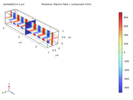
In the Settings window for Multislice, click Replace Expression in the upper-right corner of the Expression section. From the menu, choose Component 1 (comp1)>Electromagnetic Waves, Frequency Domain>Electric>Electric field - V/m>ewfd.Ex - Electric field, x component.
3
In the Electric Field (ewfd) toolbar, click  Plot. Compare the resulting plot to Figure 1.
Add Physics
Now set up the Geometrical Optics physics interface.
1
In the Home toolbar, click  Add Physics to open the Add Physics window.
2
Go to the Add Physics window.
3
In the tree, select Optics>Ray Optics>Geometrical Optics (gop).
4
Find the Physics interfaces in study subsection. In the table, clear the Solve check box for Study 1.
5
Click Add to Component 1 in the window toolbar.
6
In the Home toolbar, click  Add Physics to close the Add Physics window.
Add Study
1
In the Home toolbar, click  Add Study to open the Add Study window.
2
Go to the Add Study window.
3
Find the Physics interfaces in study subsection. In the table, clear the Solve check box for Electromagnetic Waves, Frequency Domain (ewfd).
4
Find the Studies subsection. In the Select Study tree, select Preset Studies for Selected Physics Interfaces>Ray Tracing.
5
Click Add Study in the window toolbar.
6
In the Home toolbar, click  Add Study to close the Add Study window.
Geometrical Optics (gop)
1
In the Model Builder window, under Component 1 (comp1) click Geometrical Optics (gop).
2
In the Settings window for Geometrical Optics, locate the Ray Release and Propagation section.
3
In the Maximum number of secondary rays text field, type 0.
4
Locate the Intensity Computation section. From the Intensity computation list, choose Compute intensity and power.
5
Select the Compute phase check box.
Release from Electric Field 1
1
In the Physics toolbar, click  Boundaries and choose Release from Electric Field.
2
3
In the Settings window for Release from Electric Field, locate the Initial Position section.
4
In the N text field, type 9.
5
Locate the Incident Electric Field section. From the E list, choose Electric field (ewfd/wee1).
6
Select the Use frequency from the coupled physics interface as the ray frequency check box. With this check box selected, the wavelength input in the Ray Properties node will be ignored. Instead, the vacuum wavelength will be taken directly from the previous study.
Study 2
Step 1: Ray Tracing
1
In the Model Builder window, under Study 2 click Step 1: Ray Tracing.
2
In the Settings window for Ray Tracing, locate the Study Settings section.
3
From the Time-step specification list, choose Specify maximum path length.
4
From the Length unit list, choose µm.
5
In the Lengths text field, type range(0,0.1,5).
6
Click to expand the Values of Dependent Variables section. Find the Values of variables not solved for subsection. From the Settings list, choose User controlled.
7
From the Method list, choose Solution.
8
From the Study list, choose Study 1, Wavelength Domain.
9
In the Home toolbar, click  Compute.
Results
The default plot shows the rays being released from the boundary. Modify this default plot and then add a Slice plot of the electric field.
Ray Trajectories (gop)
1
In the Settings window for 3D Plot Group, locate the Color Legend section.
2
From the Position list, choose Bottom.
Ray Trajectories 1
1
In the Model Builder window, expand the Ray Trajectories (gop) node, then click Ray Trajectories 1.
2
In the Settings window for Ray Trajectories, locate the Coloring and Style section.
3
Find the Line style subsection. From the Type list, choose Tube.
4
Find the Point style subsection. From the Type list, choose Arrow.
5
From the Arrow type list, choose Arrowhead.
Deformation 1
1
Right-click Ray Trajectories 1 and choose Deformation.
2
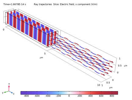
In the Settings window for Deformation, click Replace Expression in the upper-right corner of the Expression section. From the menu, choose Component 1 (comp1)>Geometrical Optics>Intensity and polarization>gop.Ex,gop.Ey,gop.Ez - Electric field.
3
Locate the Scale section.
4
Select the Scale factor check box. In the associated text field, type 5E-5.
Color Expression 1
1
In the Model Builder window, click Color Expression 1.
2
In the Settings window for Color Expression, click Replace Expression in the upper-right corner of the Expression section. From the menu, choose Component 1 (comp1)>Geometrical Optics>Intensity and polarization>Electric field - V/m>gop.Ex - Electric field, x component.
3
Locate the Coloring and Style section. Click  Change Color Table.
4
In the Color Table dialog box, select Wave>WaveLight in the tree.
5
Slice 1
1
In the Model Builder window, right-click Ray Trajectories (gop) and choose Slice.
2
In the Settings window for Slice, locate the Data section.
3
From the Dataset list, choose Study 1/Solution 1 (sol1).
4
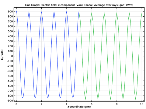
Click Replace Expression in the upper-right corner of the Expression section. From the menu, choose Component 1 (comp1)>Electromagnetic Waves, Frequency Domain>Electric>Electric field - V/m>ewfd.Ex - Electric field, x component.
5
Locate the Plane Data section. From the Plane list, choose ZX-planes.
6
In the Planes text field, type 3.
7
Click to expand the Inherit Style section. From the Plot list, choose Ray Trajectories 1.
8
In the Ray Trajectories (gop) toolbar, click  Plot. Compare the resulting plot to Figure 2.
Now add a 1D Plot Group of the x-component of the electric field.
1D Plot Group 3
1
In the Home toolbar, click  Add Plot Group and choose 1D Plot Group.
2
In the Settings window for 1D Plot Group, locate the Plot Settings section.
3
Select the x-axis label check box. In the associated text field, type z-coordinate (\mu m).
4
Select the y-axis label check box. In the associated text field, type E<sub>x</sub> (V/m).
Line Graph 1
1
Right-click 1D Plot Group 3 and choose Line Graph.
2
3
In the Settings window for Line Graph, click Replace Expression in the upper-right corner of the y-Axis Data section. From the menu, choose Component 1 (comp1)>Electromagnetic Waves, Frequency Domain>Electric>Electric field - V/m>ewfd.Ex - Electric field, x component.
4
Locate the x-Axis Data section. From the Parameter list, choose Expression.
5
In the Expression text field, type z.
Global 1
1
In the Model Builder window, right-click 1D Plot Group 3 and choose Global.
2
In the Settings window for Global, locate the Data section.
3
From the Dataset list, choose Ray 1.
4
Locate the y-Axis Data section. In the table, enter the following settings:
5
Locate the x-Axis Data section. From the Parameter list, choose Expression.
6
In the Expression text field, type gop.gopaveop1(qz).
7
Click to expand the Legends section. Clear the Show legends check box.
8
In the 1D Plot Group 3 toolbar, click  Plot. Compare the resulting plot to Figure 3.
Now use a Global Evaluation to verify that the sum of the power over all rays matches the specified input power.
Global Evaluation 2
1
In the Results toolbar, click  Global Evaluation.
2
In the Settings window for Global Evaluation, locate the Data section.
3
From the Dataset list, choose Ray 1.
4
From the Time selection list, choose Last.
5
Locate the Expressions section. In the table, enter the following settings:
6
Click  Evaluate.
The total ray power should be approximately equal to 1e-9 W, the input power specified in the Port node.