You are viewing the documentation for an older COMSOL version. The latest version is available here.
PDF

Gravitational Lensing
Introduction
This model demonstrates how the sun causes 1.75 arcseconds of deflection for rays grazing the sun’s surface as observed from Earth. Einstein predicted this value after refining his theory of relativity during World War I (Ref. 1).
Model Definition
The gravitational lensing effect is modeled using a refractive index that varies continuously in space, also known as a graded medium. The refractive index, n, depends on the gravitational constant G (SI unit: m3/(kg·s2), the solar mass m0 (SI unit: kg), the speed of light c (SI unit: m/s), and the radial distance from the center of the sun r (SI unit: m):
The gravitational constant is a built-in physical constant with the name G_const and predefined value 6.67384e-11[m^3/(kg*s^2)]. For a list of all built-in physical constants, see Physical Constants in the COMSOL Multiphysics Reference Manual.
In this example, two rays are released, which graze the surface of the sun and then continue until a distance of 150 million km is reached. At this point, the deflection angle of the rays from their initial direction is evaluated.
Results and Discussion
The angular change in the direction of the rays is plotted in Figure 1. After release, it takes the rays around 165 s to reach the sun. The rays then begin to deviate from their initial direction due to the gradient in the refractive index. The final value is about 1.75 arcseconds, consistent with Einstein’s prediction.
Figure 1: Deflection angle in arcseconds caused by the sun’s gravitational field.
Reference
1. http://en.wikipedia.org/wiki/Gravitational_lens
Application Library path: Ray_Optics_Module/Verification_Examples/gravitational_lensing
Modeling Instructions
From the File menu, choose New.
New
In the New window, click  Model Wizard.
Model Wizard
1
In the Model Wizard window, click  3D.
2
In the Select Physics tree, select Optics>Ray Optics>Geometrical Optics (gop).
3
Click Add.
4
Click  Study.
5
In the Select Study tree, select Preset Studies for Selected Physics Interfaces>Ray Tracing.
6
Global Definitions
Parameters 1
1
In the Model Builder window, under Global Definitions click Parameters 1.
2
In the Settings window for Parameters, locate the Parameters section.
3
Geometry 1
1
In the Model Builder window, under Component 1 (comp1) click Geometry 1.
2
In the Settings window for Geometry, locate the Units section.
3
From the Length unit list, choose km.
Sphere 1 (sph1)
1
In the Geometry toolbar, click  Sphere.
2
In the Settings window for Sphere, locate the Size section.
3
In the Radius text field, type r0.
Block 1 (blk1)
1
In the Geometry toolbar, click  Block.
2
In the Settings window for Block, locate the Size and Shape section.
3
In the Width text field, type 2E8.
4
In the Depth text field, type 1E7.
5
In the Height text field, type 1E7.
6
Locate the Position section. In the x text field, type 0.5E8.
7
From the Base list, choose Center.
8
Click  Build All Objects.
9
Click the  Go to Default View button in the Graphics toolbar.
10
Click the  Wireframe Rendering button in the Graphics toolbar.
Definitions
Variables 1
1
In the Model Builder window, under Component 1 (comp1) right-click Definitions and choose Variables.
2
In the Settings window for Variables, locate the Variables section.
3
Materials
Material 1 (mat1)
1
In the Model Builder window, under Component 1 (comp1) right-click Materials and choose Blank Material.
2
In the Settings window for Material, locate the Material Contents section.
3
Geometrical Optics (gop)
1
In the Model Builder window, under Component 1 (comp1) click Geometrical Optics (gop).
2
In the Settings window for Geometrical Optics, locate the Ray Release and Propagation section.
3
In the Maximum number of secondary rays text field, type 0.
Release from Grid 1
1
In the Physics toolbar, click  Global and choose Release from Grid.
Release the rays so that they barely avoid contact with the sphere that represents the sun.
2
In the Settings window for Release from Grid, locate the Initial Coordinates section.
3
In the qx,0 text field, type -0.5E8.
4
In the qy,0 text field, type -7.01E5 7.01E5.
5
Locate the Ray Direction Vector section. Specify the L0 vector as
Mesh 1
Use a Finer mesh to improve the mesh resolution in the region surrounding the sun.
1
In the Model Builder window, under Component 1 (comp1) click Mesh 1.
2
In the Settings window for Mesh, locate the Physics-Controlled Mesh section.
3
From the Element size list, choose Finer.
4
Click  Build All.
Study 1
Step 1: Ray Tracing
1
In the Model Builder window, under Study 1 click Step 1: Ray Tracing.
2
In the Settings window for Ray Tracing, locate the Study Settings section.
3
From the Time-step specification list, choose Specify maximum path length.
4
From the Length unit list, choose km.
5
Click  Range.
6
In the Range dialog box, choose Number of values from the Entry method list.
7
In the Stop text field, type 2E8.
8
In the Number of values text field, type 100.
9
Click Replace.
Solution 1 (sol1)
1
In the Study toolbar, click  Show Default Solver.
2
In the Model Builder window, expand the Solution 1 (sol1) node, then click Time-Dependent Solver 1.
3
In the Settings window for Time-Dependent Solver, click to expand the Time Stepping section.
4
From the Maximum step constraint list, choose Constant.
5
In the Maximum step text field, type 1.
6
In the Study toolbar, click  Compute.
Results
Ray Trajectories (gop)
In the Model Builder window, expand the Ray Trajectories (gop) node.
Color Expression 1
1
In the Model Builder window, expand the Results>Ray Trajectories (gop)>Ray Trajectories 1 node, then click Color Expression 1.
2
In the Settings window for Color Expression, locate the Expression section.
3
In the Expression text field, type asin(gop.niy).
4
From the Unit list, choose arcsec.
5
In the Ray Trajectories (gop) toolbar, click  Plot.
Ray Evaluation 1
1
In the Results toolbar, click  More Derived Values and choose Other>Ray Evaluation.
2
In the Settings window for Ray Evaluation, locate the Data section.
3
From the Time selection list, choose Last.
4
Locate the Expression section. In the Expression text field, type asin(gop.niy).
5
From the Unit list, choose arcsec.
6
Click  Evaluate.
Compare the resulting values to Einstein’s prediction of 1.75 arcseconds.
Deviation from Initial Direction
1
In the Results toolbar, click  1D Plot Group.
2
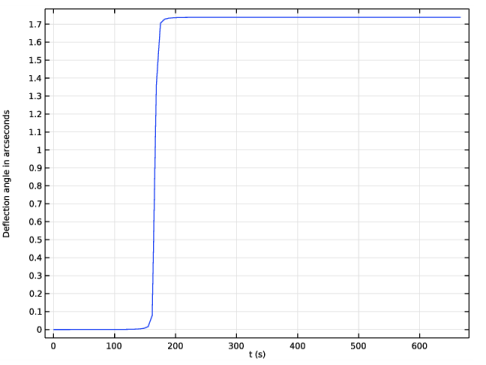
In the Settings window for 1D Plot Group, type Deviation from Initial Direction in the Label text field.
3
Locate the Data section. From the Dataset list, choose Ray 1.
4
Click to expand the Title section. From the Title type list, choose None.
5
Locate the Plot Settings section.
6
Select the y-axis label check box. In the associated text field, type Deflection angle in arcseconds.
Ray 1
1
In the Deviation from Initial Direction toolbar, click  More Plots and choose Ray.
2
In the Settings window for Ray, locate the y-Axis Data section.
3
In the Expression text field, type abs(asin(gop.niy)).
4
From the Unit list, choose arcsec.
5
In the Deviation from Initial Direction toolbar, click  Plot.
6
Locate the Data Series Operation section. From the Operation list, choose Average.
7
In the Deviation from Initial Direction toolbar, click  Plot. Compare the resulting plot to Figure 1.