You are viewing the documentation for an older COMSOL version. The latest version is available here.
PDF

Cross Grating Échelle Spectrograph
Introduction
This tutorial demonstrates the use of a Cross Grating in an échelle spectrograph. A cross grating is a periodic surface with two directions of periodicity can be specified. In this model, the cross grating is used in high order in one direction, and in first order in the orthogonal (“cross”) direction. By this means, a two-dimensional cross-dispersed spectrum can be produced with a single grating.
Another cross-dispersed spectrograph is the White Pupil Échelle Spectrograph. This model utilizes two separate échelle and cross-dispersion Grating features in order to create a two-dimensional spectral format.
Model Definition
An example of a cross grating spectrograph is described in Ref. 1. The optical layout used in this tutorial follows this example with some modifications.
The surface used to define the Cross Grating feature is shown in Figure 1. Like the Grating feature, the grating orientation may be specified in one of several ways. For this model, we choose to Specific direction of periodicity, with that direction set to Parallel to reference edge. In this figure, the grating surface normal is shown in blue, the direction of échelle dispersion is red, and the cross-dispersion direction is green.
Figure 1: The Cross Grating showing the surface normal and directions of periodicity. The incident rays are traveling in the +z direction.
The geometry for the model, including the camera objective, can be inserted from a predefined sequence. Full instructions for creating the geometry sequence are given in Appendix — Geometry Instructions. An overview of the objective lens can be found in the Petzval Lens tutorial. The parameters used to create the sequence are listed in Table 1. Details of the collimating doublet lens used in this model are from Ref. 2.
λmid
Tech
σech
μm
Échelle-dispersion definitions:
θB
Δθ
γ
R1,doub
R2,doub
R3,doub
Tc1,doub
Tc2,doub
d0doub
BFLdoub
After insertion, the geometry sequence should look like Figure 2. Note that the geometry is fully parameterized. Therefore, a change in the cross grating properties will cause the geometry to be updated.
The mesh for this simulation is shown in Figure 3. Because this model does not include any other physics, an undeformed geometry can be used to trace rays. Therefore, only a small refinement of the default Physics-controlled mesh is necessary.
The remaining model parameters are listed in Table 2. Note that the λnom is a nominal wavelength only. It is used to define the order m in which this wavelength appears. That is, λnom is used to control the range of the Parametric Sweep. The expressions found in Table 2 give the blaze wavelength and free spectral ranges for any given order.
Figure 2: The Cross Grating Échelle Spectrograph geometry sequence.
Figure 3: The Cross Grating Échelle Spectrograph mesh.
λnom
Nhex
10
Nlam
fcol
15.0 mm
6.67
NA
0.5/F
0.075
Tech
50.0 /mm
σech
20 μm
mλ
35466058 nm
68
521.560 nm
ΔλFSR
7.670 nm
λmin
λmax
λstep
Results and Discussion
A Parametric Sweep over three orders spanning a nominal 100 nm has been made. A Release from Point is used to generate a conical distribution of rays uniformly covering the collimated beam diameter. Figure 4 shows a plan view of the resulting ray trace. A perspective view is seen in Figure 5.
The échelle diagram is seen in Figure 6. The wavelength range spans from 469.7 nm to 576.6 nm in orders m = 75 to 62.
The image quality at each wavelength can be seen in Figure 7. The color expression used in this plot is the release angle relative to the chief ray.
Figure 4: Ray trace through the Cross Grating Échelle Spectrograph. This plan view shows the direction of cross-dispersion.
Figure 5: A perspective view of a ray trace through the Cross Grating Échelle Spectrograph.
Figure 6: The Cross Grating Échelle Spectrograph échelle diagram.
Figure 7: A spot diagram for the Cross Grating Échelle Spectrograph.
References
1. D. Thomae, T. Honle, M. Kraus, V. Bagusat, A. Deparnay, R. Bruning, and R. Brunner. “Compact echelle spectrometer employing a cross-grating,” Applied Optics, vol. 57, no. 25, pp. 2109–7116, 2018.
2. M.J. Kidger, Fundamental Optical Design, Bellingham WA, USA: SPIE Press, 2001.
Application Library path: Ray_Optics_Module/Spectrometers_and_Monochromators/cross_grating_echelle_spectrograph
Modeling Instructions
From the File menu, choose New.
New
In the New window, click  Model Wizard.
Model Wizard
1
In the Model Wizard window, click  3D.
2
In the Select Physics tree, select Optics>Ray Optics>Geometrical Optics (gop).
3
Click Add.
4
Click  Study.
5
In the Select Study tree, select Preset Studies for Selected Physics Interfaces>Ray Tracing.
6
Global Definitions
Parameters 1: Geometry
1
In the Model Builder window, under Global Definitions click Parameters 1.
2
In the Settings window for Parameters, type Parameters 1: Geometry in the Label text field. The geometry parameters will be added when the geometry sequence is inserted below.
Parameters 2: Model
1
In the Home toolbar, click  Parameters and choose Add>Parameters.
2
In the Settings window for Parameters, type Parameters 2: Model in the Label text field.
3
Locate the Parameters section. Click  Load from File.
4
Cross Grating Échelle Spectrograph Geometry Sequence
Insert the prepared geometry sequence from file. You can read the instructions for creating the geometry in the appendix. Following insertion, the full geometry definition will be available in the Parameters node.
1
In the Model Builder window, under Component 1 (comp1) click Geometry 1.
2
In the Settings window for Geometry, type Cross Grating Échelle Spectrograph Geometry Sequence in the Label text field.
3
In the Geometry toolbar, click Insert Sequence and choose Insert Sequence.
4
Browse to the model’s Application Libraries folder and double-click the file cross_grating_echelle_spectrograph_geom_sequence.mph.
5
In the Geometry toolbar, click  Build All.
6
Click the  Orthographic Projection button in the Graphics toolbar.
7
In the Graphics window toolbar, clicknext to  Go to Default View, then choose Go to ZX View.
8
Click the  Zoom Extents button in the Graphics toolbar. Orient the view to place the z-axis (optical axis) horizontal and the y-axis vertical. Compare the resulting geometry to Figure 2.
Materials
Load the materials that are used in this model.
Add Material
1
In the Home toolbar, click  Add Material to open the Add Material window.
2
Go to the Add Material window.
3
In the tree, select Optical>Schott Glass>Schott N-BK7 Glass.
4
Click Add to Component in the window toolbar.
5
In the tree, select Optical>Schott Glass>Schott N-KZFS5 Glass.
6
Click Add to Component in the window toolbar.
7
In the tree, select Optical>Schott Glass>Schott N-SK2 Glass.
8
Click Add to Component in the window toolbar.
9
In the tree, select Optical>Schott Glass>Schott N-SF5 Glass.
10
Click Add to Component in the window toolbar.
11
In the tree, select Optical>CDGM Glass>CDGM H-ZF39 Glass.
12
Click Add to Component in the window toolbar.
13
In the tree, select Optical>Schott Glass>Schott N-SK11 Glass.
14
Click Add to Component in the window toolbar.
15
In the Home toolbar, click  Add Material to close the Add Material window.
Now, assign these materials to the appropriate domains using the predefined selections.
Materials
Schott N-BK7 Glass (mat1)
1
In the Model Builder window, under Component 1 (comp1)>Materials click Schott N-BK7 Glass (mat1).
2
In the Settings window for Material, locate the Geometric Entity Selection section.
3
From the Selection list, choose Lens Material 1.
Schott N-KZFS5 Glass (mat2)
1
In the Model Builder window, click Schott N-KZFS5 Glass (mat2).
2
In the Settings window for Material, locate the Geometric Entity Selection section.
3
From the Selection list, choose Lens Material 2.
Schott N-SK2 Glass (mat3)
1
In the Model Builder window, click Schott N-SK2 Glass (mat3).
2
In the Settings window for Material, locate the Geometric Entity Selection section.
3
From the Selection list, choose Lens Material 3.
Schott N-SF5 Glass (mat4)
1
In the Model Builder window, click Schott N-SF5 Glass (mat4).
2
In the Settings window for Material, locate the Geometric Entity Selection section.
3
From the Selection list, choose Lens Material 4.
CDGM H-ZF39 Glass (mat5)
1
In the Model Builder window, click CDGM H-ZF39 Glass (mat5).
2
In the Settings window for Material, locate the Geometric Entity Selection section.
3
From the Selection list, choose Element 1 (Collimator Lens).
Schott N-SK11 Glass (mat6)
1
In the Model Builder window, click Schott N-SK11 Glass (mat6).
2
In the Settings window for Material, locate the Geometric Entity Selection section.
3
From the Selection list, choose Element 2 (Collimator Lens).
Geometrical Optics (gop)
1
In the Model Builder window, under Component 1 (comp1) click Geometrical Optics (gop).
2
In the Settings window for Geometrical Optics, locate the Ray Release and Propagation section.
3
From the Wavelength distribution of released rays list, choose Polychromatic, specify vacuum wavelength.
4
In the Maximum number of secondary rays text field, type 0.
5
Locate the Material Properties of Exterior and Unmeshed Domains section. From the Optical dispersion model list, choose Air, Edlen (1953). The collimator lens and camera objective have been optimized for use in air.
6
Locate the Additional Variables section. Select the Compute optical path length check box. The optical path length will be used to distinguish rays on the image plane from other rays which also intersect the same plane.
Medium Properties 1
1
In the Model Builder window, under Component 1 (comp1)>Geometrical Optics (gop) click Medium Properties 1.
2
In the Settings window for Medium Properties, locate the Medium Properties section.
3
From the Refractive index of domains list, choose Get dispersion model from material. The materials previously loaded contain the coefficients for the optical dispersions models that are used to compute the wavelength dependent refractive indices.
Material Discontinuity 1
1
In the Model Builder window, click Material Discontinuity 1.
2
In the Settings window for Material Discontinuity, locate the Rays to Release section.
3
From the Release reflected rays list, choose Never. Scattered light is not considered in this model.
Cross Grating 1
1
In the Physics toolbar, click  Boundaries and choose Cross Grating.
2
In the Settings window for Cross Grating, locate the Boundary Selection section.
3
From the Selection list, choose Cross Grating Surface.
4
Locate the Device Properties section. From the Rays to release list, choose Reflected.
5
In the d1 text field, type sigma_ech.
6
In the d2 text field, type sigma_xdp.
7
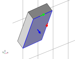
Locate the Grating Orientation 1 section. From the Direction of periodicity 1 list, choose Parallel to reference edge.
8
Locate the Reference Edge Selection, Direction 1 section. Click to select the  Activate Selection toggle button.
9
10
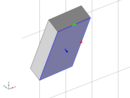
Locate the Grating Orientation 2 section. From the Direction of periodicity 2 list, choose Parallel to reference edge.
11
Locate the Reference Edge Selection, Direction 2 section. Click to select the  Activate Selection toggle button.
12
Diffraction Order (m = 0, n = 0)
1
In the Model Builder window, expand the Cross Grating 1 node, then click Diffraction Order (m = 0, n = 0).
2
In the Settings window for Diffraction Order, locate the Device Properties section.
3
In the m text field, type m. The echelle order number is computed in the Parameters 2: Model node using the nominal wavelength lam_nom.
4
In the n text field, type 1. The cross-dispersion will be in the first order.
Obstructions
1
In the Physics toolbar, click  Boundaries and choose Wall.
2
In the Settings window for Wall, type Obstructions in the Label text field.
3
Locate the Boundary Selection section. From the Selection list, choose Obstructions.
4
Locate the Wall Condition section. From the Wall condition list, choose Disappear. Note that in this model, the internal aperture stop of the Petzval lens will be ignored.
Image Plane
1
In the Physics toolbar, click  Boundaries and choose Wall.
2
In the Settings window for Wall, type Image Plane in the Label text field.
3
Locate the Boundary Selection section. From the Selection list, choose Image Plane. The default Wall condition Freeze will be applied to rays that intersect the image surface.
Release from Point 1
1
In the Physics toolbar, click  Points and choose Release from Point.
2
In the Settings window for Release from Point, locate the Point Selection section.
3
From the Selection list, choose Entrance slit (point).
4
Locate the Ray Direction Vector section. From the Ray direction vector list, choose Conical.
5
From the Conical distribution list, choose Hexapolar.
6
In the Nθ text field, type N_hex. The number of hexapolar angles was defined in the Parameters 2: Model node.
7
Specify the r vector as
8
In the α text field, type atan(NA).
9
Locate the Vacuum Wavelength section. From the Distribution function list, choose List of values.
10
In the Values text field, type range(lam_min,lam_step,lam_max). These wavelengths span one free spectral range centered on the blaze wavelength. The values are also defined in the Parameters node.
Definitions
In the following steps Nonlocal Couplings are used to allow the three corners of the image surface to be used to define an Intersection Point 3D dataset.
Average 1 (aveop1)
1
In the Definitions toolbar, click  Nonlocal Couplings and choose Average.
2
In the Settings window for Average, locate the Source Selection section.
3
From the Geometric entity level list, choose Point.
4
Average 2 (aveop2)
1
In the Definitions toolbar, click  Nonlocal Couplings and choose Average.
2
In the Settings window for Average, locate the Source Selection section.
3
From the Geometric entity level list, choose Point.
4
Average 3 (aveop3)
1
In the Definitions toolbar, click  Nonlocal Couplings and choose Average.
2
In the Settings window for Average, locate the Source Selection section.
3
From the Geometric entity level list, choose Point.
4
Mesh 1
1
In the Model Builder window, under Component 1 (comp1) click Mesh 1.
2
In the Settings window for Mesh, locate the Physics-Controlled Mesh section.
3
From the Element size list, choose Fine. Refine the mesh slightly to reduce discretization errors.
4
Click  Build All. The mesh should appear like Figure 3.
Study 1
Step 1: Ray Tracing
1
In the Model Builder window, under Study 1 click Step 1: Ray Tracing.
2
In the Settings window for Ray Tracing, locate the Study Settings section.
3
From the Time-step specification list, choose Specify maximum path length.
4
From the Length unit list, choose mm.
5
In the Lengths text field, type 0 450. This path length is sufficient to ensure that all rays make it to the image plane.
Add a parametric sweep to trace rays in several orders.
Parametric Sweep
1
In the Study toolbar, click  Parametric Sweep.
2
In the Settings window for Parametric Sweep, locate the Study Settings section.
3
4
5
6
In the Study toolbar, click  Compute.
Results
Ray Diagram
Use the default Ray Trajectories plot as a starting point for a Ray Diagram.
1
In the Settings window for 3D Plot Group, type Ray Diagram in the Label text field.
2
Click to expand the Title section. From the Title type list, choose None.
3
Locate the Color Legend section. Select the Show maximum and minimum values check box.
4
Select the Show units check box.
5
From the Position list, choose Bottom.
6
Click to expand the Number Format section. Select the Manual color legend settings check box.
7
In the Precision text field, type 4.
Ray Trajectories 1
1
In the Model Builder window, expand the Ray Diagram node, then click Ray Trajectories 1.
2
In the Settings window for Ray Trajectories, locate the Data section.
3
From the Dataset list, choose Ray 1.
4
From the Parameter value (lam_nom (nm)) list, choose 475.
Color Expression 1
1
In the Model Builder window, expand the Ray Trajectories 1 node, then click Color Expression 1.
2
In the Settings window for Color Expression, locate the Expression section.
3
In the Expression text field, type gop.lambda0.
4
From the Unit list, choose nm.
5
Locate the Coloring and Style section. Click  Change Color Table.
6
In the Color Table dialog box, select Rainbow>Spectrum in the tree.
7
Filter 1
1
In the Model Builder window, click Filter 1.
2
In the Settings window for Filter, locate the Ray Selection section.
3
From the Rays to render list, choose Fraction.
4
In the Fraction of rays text field, type .05. Show only 5% of the rays to improve the rendering.
Ray Trajectories 2
1
In the Model Builder window, under Results>Ray Diagram right-click Ray Trajectories 1 and choose Duplicate.
2
In the Settings window for Ray Trajectories, locate the Data section.
3
From the Parameter value (lam_nom (nm)) list, choose 525.
4
Click to expand the Inherit Style section. From the Plot list, choose Ray Trajectories 1.
Ray Trajectories 3
1
Right-click Ray Trajectories 2 and choose Duplicate.
2
In the Settings window for Ray Trajectories, locate the Data section.
3
From the Parameter value (lam_nom (nm)) list, choose 575.
Surface 1
1
In the Model Builder window, right-click Ray Diagram and choose Surface.
2
In the Settings window for Surface, locate the Coloring and Style section.
3
From the Coloring list, choose Uniform.
4
From the Color list, choose Gray.
Transparency 1
1
Right-click Surface 1 and choose Transparency.
2
In the Ray Diagram toolbar, click  Plot.
3
Click the  Zoom Extents button in the Graphics toolbar. Compare the resulting image to Figure 4. Orient the view to match Figure 5 to show the all the rays.
Intersection Point 3D 1
1
In the Results toolbar, click  More Datasets and choose Intersection Point 3D. In the following steps, use the Nonlocal Couplings defined above to create a dataset that intersects the image plane.
2
In the Settings window for Intersection Point 3D, locate the Surface section.
3
From the Plane entry method list, choose Three points.
4
In row Point 1, set x to aveop1(x).
5
In row Point 1, set y to aveop1(y).
6
In row Point 1, set z to aveop1(z).
7
In row Point 2, set x to aveop2(x).
8
In row Point 2, set y to aveop2(y).
9
In row Point 2, set z to aveop2(z).
10
In row Point 3, set x to aveop3(x).
11
In row Point 3, set y to aveop3(y).
12
In row Point 3, set z to aveop3(z).
The Intersection Point 3D dataset can be used together with the Spot Diagram plot to create two plots. The first, an Échelle diagram, shows the absolute location of all rays in the image surface. The second, shows the monochromatic spots.
Échelle Diagram
1
In the Results toolbar, click  2D Plot Group.
2
In the Settings window for 2D Plot Group, type Échelle Diagram in the Label text field.
3
Locate the Data section. From the Dataset list, choose None.
4
Click to expand the Title section. From the Title type list, choose None.
5
Locate the Color Legend section. Select the Show maximum and minimum values check box.
6
Select the Show units check box.
7
From the Position list, choose Bottom.
8
Click to expand the Number Format section. Select the Manual color legend settings check box.
9
In the Precision text field, type 4.
Spot Diagram 1
1
In the Échelle Diagram toolbar, click  More Plots and choose Spot Diagram.
2
In the Settings window for Spot Diagram, locate the Data section.
3
From the Image surface list, choose Intersection Point 3D 1.
4
Locate the Filters section.
5
Select the Filter by additional logical expression check box. In the associated text field, type comp1.gop.L>100[mm]. Because the plane intersecting the image surface also passes through ray trajectories before they reach the image plane, these ray intersections must be removed from the plot.
6
Locate the Layout section. From the Spot arrangement list, choose Single plot.
7
Click to expand the Annotations section. Clear the Show spot size check box.
8
Locate the Coloring and Style section. Select the Radius scale factor check box.
Color Expression 1
1
Right-click Spot Diagram 1 and choose Color Expression.
2
In the Settings window for Color Expression, locate the Expression section.
3
In the Expression text field, type gop.lambda0.
4
From the Unit list, choose nm.
5
In the Échelle Diagram toolbar, click  Plot.
6
Click the  Zoom Extents button in the Graphics toolbar. Compare this figure to Figure 6.
In the following steps a standard spot diagram will be created.
Spot Diagram
1
In the Home toolbar, click  Add Plot Group and choose 2D Plot Group.
2
In the Settings window for 2D Plot Group, type Spot Diagram in the Label text field.
3
Locate the Data section. From the Dataset list, choose None.
4
Locate the Color Legend section. Select the Show maximum and minimum values check box.
5
Select the Show units check box.
6
From the Position list, choose Bottom.
Spot Diagram 1
1
In the Spot Diagram toolbar, click  More Plots and choose Spot Diagram.
2
In the Settings window for Spot Diagram, locate the Data section.
3
From the Image surface list, choose Intersection Point 3D 1.
4
Locate the Filters section.
5
Select the Filter by additional logical expression check box. In the associated text field, type comp1.gop.L>100[mm].
6
Locate the Layout section. From the Spot arrangement list, choose Sort by wavelength.
7
From the Layout list, choose Rectangular grid.
8
In the Number of columns text field, type 5.
9
Locate the Annotations section. Select the Show wavelength check box.
Color Expression 1
1
Right-click Spot Diagram 1 and choose Color Expression.
2
In the Settings window for Color Expression, locate the Expression section.
3
In the Expression text field, type at(0,gop.phic). This is the angle from the cone axis at the entrance slit.
4
In the Unit field, type deg.
5
In the Spot Diagram toolbar, click  Plot.
6
Click the  Show Grid button in the Graphics toolbar.
7
Click the  Zoom Extents button in the Graphics toolbar. Compare this figure to Figure 7.
Appendix — Geometry Instructions
From the File menu, choose New.
New
In the New window, click  Model Wizard.
Model Wizard
1
In the Model Wizard window, click  3D.
2
Global Definitions
Parameters 1
1
In the Model Builder window, under Global Definitions click Parameters 1.
2
In the Settings window for Parameters, locate the Parameters section.
3
Click  Load from File.
4
Browse to the model’s Application Libraries folder and double-click the file cross_grating_echelle_spectrograph_geom_sequence_parameters.txt.
Geometry 1
1
In the Model Builder window, under Component 1 (comp1) click Geometry 1.
2
In the Settings window for Geometry, locate the Units section.
3
From the Length unit list, choose mm.
Entrance slit (point)
1
In the Geometry toolbar, click  More Primitives and choose Point.
2
In the Settings window for Point, type Entrance slit (point) in the Label text field.
3
Locate the Selections of Resulting Entities section. Select the Resulting objects selection check box.
Part Libraries
1
In the Geometry toolbar, click  Parts and choose Part Libraries.
2
In the Model Builder window, click Geometry 1.
3
In the Part Libraries window, select Ray Optics Module>3D>Doublet and Triplet Lenses>spherical_doublet_lens_3d in the tree.
4
Click  Add to Geometry.
5
In the Select Part Variant dialog box, select Contact doublet, specify clear aperture diameter in the Select part variant list.
6
Geometry 1
Collimator Lens
The doublet lens used in this model is a Fraunhofer doublet from Ref. 2, pg 172. The parameters were defined in the Parameters node.
1
In the Model Builder window, under Component 1 (comp1)>Geometry 1 click Spherical Doublet Lens 3D 1 (pi1).
2
In the Settings window for Part Instance, type Collimator Lens in the Label text field.
3
Locate the Input Parameters section. In the table, enter the following settings:
4
Locate the Position and Orientation of Output section. Find the Displacement subsection. In the zw text field, type BFL_doub.
5
Click to expand the Domain Selections section. In the table, select the Keep check boxes for Element 1 and Element 2.
In the following steps, the orientation of the cross grating is defined using a series of Work Planes.
Cross Grating Incoming Reference
1
In the Geometry toolbar, click  Work Plane.
2
In the Settings window for Work Plane, type Cross Grating Incoming Reference in the Label text field.
3
Locate the Plane Definition section. From the Plane type list, choose Normal vector.
4
Find the Normal vector subsection. In the y text field, type 1.
5
In the z text field, type 0.
6
Find the Point on plane subsection. In the z text field, type 200.
Cross Grating Facet Tangent
1
In the Geometry toolbar, click  Work Plane.
2
In the Settings window for Work Plane, type Cross Grating Facet Tangent in the Label text field.
3
Locate the Plane Definition section. From the Plane type list, choose Transformed.
4
From the Work plane to transform list, choose Cross Grating Incoming Reference (wp1).
5
Find the Rotation subsection. In the Rotation angle text field, type theta_xdp-gamma.
Cross Grating Facet Normal
1
In the Geometry toolbar, click  Work Plane.
2
In the Settings window for Work Plane, type Cross Grating Facet Normal in the Label text field.
3
Locate the Plane Definition section. From the Plane type list, choose Transformed.
4
From the Work plane to transform list, choose Cross Grating Facet Tangent (wp2).
5
Find the Rotation subsection. From the Axis type list, choose yw-axis.
6
In the Rotation angle text field, type 90.
Cross Grating Surface
1
In the Geometry toolbar, click  Work Plane.
2
In the Settings window for Work Plane, type Cross Grating Surface in the Label text field.
3
Locate the Plane Definition section. From the Plane type list, choose Transformed.
4
From the Work plane to transform list, choose Cross Grating Facet Normal (wp3).
5
Find the Rotation subsection. From the Axis type list, choose yw-axis.
6
In the Rotation angle text field, type theta_B+dtheta.
7
Locate the Selections of Resulting Entities section. Select the Resulting objects selection check box. The grating surface will be defined on this work plane.
Cross Grating Surface (wp4)>Plane Geometry
In the Model Builder window, click Plane Geometry.
Cross Grating Surface (wp4)>Rectangle 1 (r1)
1
In the Work Plane toolbar, click  Rectangle.
2
In the Settings window for Rectangle, locate the Size and Shape section.
3
In the Width text field, type 50.0.
4
In the Height text field, type 25.0.
5
Locate the Position section. From the Base list, choose Center.
Cross Grating
1
In the Model Builder window, right-click Geometry 1 and choose Extrude.
2
In the Settings window for Extrude, type Cross Grating in the Label text field.
3
Locate the Distances section. In the table, enter the following settings:
4
Select the Reverse direction check box.
Cross Grating Outgoing Reference
1
In the Geometry toolbar, click  Work Plane.
2
In the Settings window for Work Plane, type Cross Grating Outgoing Reference in the Label text field.
3
Locate the Plane Definition section. From the Plane type list, choose Transformed.
4
From the Work plane to transform list, choose Cross Grating Facet Normal (wp3).
5
Find the Rotation subsection. From the Axis type list, choose xw-axis.
6
In the Rotation angle text field, type theta_xdp+gamma.
Petzval Lens Geometry Sequence
The objective lens used in the spectrograph can be inserted from file using a prepared geometry sequence. For detailed instructions on creating this geometry see the appendix of the Petzval Lens tutorial.
1
In the Geometry toolbar, click Insert Sequence and choose Insert Sequence.
2
Browse to the model’s Application Libraries folder and double-click the file cross_grating_echelle_spectrograph_petzval_lens_geom_sequence.mph.
Now, position the lens in the spectrograph geometry using the predefined work planes.
Lens 1 (pi2)
1
In the Model Builder window, click Lens 1 (pi2).
2
In the Settings window for Part Instance, locate the Position and Orientation of Output section.
3
Find the Coordinate system to match subsection. From the Work plane list, choose Cross Grating Outgoing Reference (wp5).
4
Find the Displacement subsection. In the yw text field, type -1.5[mm].
5
In the zw text field, type 75.0[mm].
Group 1 Aperture (pi9), Group 2 Aperture (pi10), Group 3 Aperture (pi11)
1
In the Model Builder window, under Component 1 (comp1)>Geometry 1, Ctrl-click to select Group 1 Aperture (pi9), Group 2 Aperture (pi10), and Group 3 Aperture (pi11).
2
Right-click and choose Disable. These apertures are not needed in this model.
Scale 1 (sca1)
1
In the Geometry toolbar, click  Transforms and choose Scale.
2
Select the objects pi2, pi3, pi4, pi5, pi6, pi7, and pi8 only.
3
In the Settings window for Scale, locate the Scale Factor section.
4
In the Factor text field, type 0.667. The focal length of the Petzval lens is reduced to 66.7 mm.
5
Locate the Coordinate System section. From the Take work plane from list, choose Lens 1 (pi2).
6
From the Work plane list, choose Surface 1 vertex intersection (wp1).
Cross Grating (ext1)
1
In the Model Builder window, click Cross Grating (ext1).
2
In the Settings window for Extrude, locate the Selections of Resulting Entities section.
3
Find the Cumulative selection subsection. From the Contribute to list, choose Lens Material 1.
Global Definitions
Parameters 1
1
In the Model Builder window, under Global Definitions click Parameters 1.
2
In the Settings window for Parameters, locate the Parameters section.
3
4
Right-click Global Definitions>Parameters 1 and choose Build All Objects.
5
Click the  Orthographic Projection button in the Graphics toolbar.
6
In the Graphics window toolbar, clicknext to  Go to Default View, then choose Go to ZX View.
7
Click the  Zoom Extents button in the Graphics toolbar. Compare the resulting image to Figure 2.