PDF

Two-Arm Helical Antenna
Introduction
A helical antenna has two major modes. One is normal mode and the other is axial mode. When the helical antenna is operating at the normal mode, its far-field radiation pattern is similar to the torus-shaped pattern of a classic dipole antenna. At the axial mode, the helical antenna is resonant at a much higher frequency band than at the normal mode operation; it works similarly to an end-fire array along the z-axis, generating a directive radiation pattern. This example analyzes a helical antenna at these two different modes. The S-parameters and far-field patterns are calculated at both operating modes, 385 MHz and 4.77 GHz.
Figure 1: Each end of the two-arm helix is connected to a coaxial cable feed and ground plate. A region of free space bounded by a perfectly matched layer (PML) surrounding the antenna. The ground plate and PML are partially visualized.
Model Definition
The model consists of a two-arm helix radiator, a circular ground plate, a tuning stub, a coaxial cable, and a perfectly matched layer (PML) enclosing an air region. One bottom end of the helix arm is connected to the inner conductor pin from the coaxial cable and the other end is shorted to the ground plate. Two helix structures are wound along the z-axis and meet at the top end. The impedance of a single-helix antenna is much lower than 50 Ω when it is resonant at the normal mode. By adding an additional helix shorted to the ground, the antenna works as a folded antenna which is known for its four times bigger input resistance than that of a same size dipole antenna, and the low impedance can be adjusted close to the reference impedance of the coaxial cable, 50 Ω. An additional impedance matching stub for the axial mode is located at the center of the ground plate.
All metal parts in this example are modeled as perfect electric conductors (PEC) and their interior domains are not included in the analysis. The space between the inner and outer conductor of the coaxial cable is filled with polytetrafluoroethylene (PTFE), a material with relative permittivity εr = 2.1. A coaxial type lumped port is used to excite the antenna.
All domains except the PML are meshed by a tetrahedral mesh with approximately five elements per wavelength. The helix and coaxial cable are meshed more finely to provide good resolution of the curved surfaces. The PML is swept with a total of five elements along the radial direction.
The ground plate, the PML sphere shell, and the maximum mesh size are adjusted automatically as a function of wavelength for each helical antenna mode.
Results and Discussion
The antenna is analyzed for two operating modes. Figure 2 and Figure 3 show the log-scaled electric field norm describing the field intensity around the antenna at the axial mode and normal mode, respectively. Figure 4 shows a polar plot of 2D radiation patterns in the yz-plane for both modes. A directional radiation pattern is observed at the axial mode while the radiation pattern at the normal mode resembles the E-plane pattern of a classic dipole antenna. The 3D far-field radiation pattern for each mode is also plotted in Figure 5 and Figure 6. The S-parameters for both modes are less than 10 dB.
Figure 2: Log-scaled electric field magnitude around the antenna at 4.77 GHz.
Figure 3: Log-scaled electric field magnitude around the antenna at 385 MHz.
Figure 4: Polar plot of the far-field pattern in the yz-plane.
Figure 5: The 3D far-field pattern looks like that of an end-fire array along the z-axis backed by a ground plane.
Figure 6: The torus-shaped 3D far-field pattern resembles that of a dipole antenna.
Notes About the COMSOL Implementation
Due to the complexity of the geometry and mesh, more than 7 GB RAM is required to run this example.
Application Library path: RF_Module/Antennas/helical_antenna
Modeling Instructions
From the File menu, choose New.
New
In the New window, click  Model Wizard.
Model Wizard
1
In the Model Wizard window, click  3D.
2
In the Select Physics tree, select Radio Frequency>Electromagnetic Waves, Frequency Domain (emw).
3
Click Add.
4
Click  Study.
5
In the Select Study tree, select General Studies>Frequency Domain.
6
Global Definitions
Parameters 1
1
In the Model Builder window, under Global Definitions click Parameters 1.
2
In the Settings window for Parameters, locate the Parameters section.
3
Click  Load from File.
4
Here, c_const is a predefined COMSOL constant for the speed of light in vacuum.
Study 1
Step 1: Frequency Domain
1
In the Model Builder window, under Study 1 click Step 1: Frequency Domain.
2
In the Settings window for Frequency Domain, locate the Study Settings section.
3
In the Frequencies text field, type f0.
Geometry 1
1
In the Model Builder window, under Component 1 (comp1) click Geometry 1.
2
In the Settings window for Geometry, locate the Units section.
3
From the Length unit list, choose mm.
Create a helix with the specified parameters.
Helix 1 (hel1)
1
In the Geometry toolbar, click  Helix.
2
In the Settings window for Helix, locate the Size and Shape section.
3
In the Number of turns text field, type n_turn.
4
In the Major radius text field, type r_helix.
5
In the Minor radius text field, type 1.
6
In the Axial pitch text field, type a_pitch.
Add a torus connected to one end the helix.
Torus 1 (tor1)
1
In the Geometry toolbar, click  Torus.
2
In the Settings window for Torus, locate the Size and Shape section.
3
In the Major radius text field, type r_helix/2.
4
In the Minor radius text field, type 1.
5
In the Revolution angle text field, type 180.
6
Locate the Position section. In the x text field, type r_helix/2.
7
In the z text field, type a_pitch*n_turn.
Add a cylinder for the extended part of the coaxial cable inner conductor and ground pin.
Cylinder 1 (cyl1)
1
In the Geometry toolbar, click  Cylinder.
2
In the Settings window for Cylinder, locate the Size and Shape section.
3
In the Radius text field, type 0.635.
4
In the Height text field, type l_pin.
5
Locate the Position section. In the x text field, type r_helix.
6
In the z text field, type -l_pin.
Add a sphere for the solder ball.
Sphere 1 (sph1)
1
In the Geometry toolbar, click  Sphere.
2
In the Settings window for Sphere, locate the Size section.
3
In the Radius text field, type 3.6.
4
Locate the Position section. In the x text field, type r_helix.
5
In the z text field, type 1.5.
6
Click  Build Selected.
Generate the other arm of the helix by rotating the first arm.
Rotate 1 (rot1)
1
In the Geometry toolbar, click  Transforms and choose Rotate.
2
Click in the Graphics window and then press Ctrl+A to select all objects.
3
In the Settings window for Rotate, locate the Input section.
4
Select the Keep input objects check box.
5
Locate the Rotation section. In the Angle text field, type 180.
Create a union of all geometries to remove unnecessary interior boundaries.
Union 1 (uni1)
1
In the Geometry toolbar, click  Booleans and Partitions and choose Union.
2
Click in the Graphics window and then press Ctrl+A to select all objects.
3
In the Settings window for Union, locate the Union section.
4
Clear the Keep interior boundaries check box.
5
Click  Build Selected.
Add a cylinder for the coaxial cable inner conductor.
Cylinder 2 (cyl2)
1
In the Geometry toolbar, click  Cylinder.
2
In the Settings window for Cylinder, locate the Size and Shape section.
3
In the Radius text field, type 0.635.
4
In the Height text field, type h_ground.
5
Locate the Position section. In the x text field, type r_helix.
6
In the z text field, type -h_ground-l_pin.
Add a cylinder for the coaxial cable outer conductor.
Cylinder 3 (cyl3)
1
In the Geometry toolbar, click  Cylinder.
2
In the Settings window for Cylinder, locate the Size and Shape section.
3
In the Radius text field, type 2.05.
4
In the Height text field, type h_ground.
5
Locate the Position section. In the x text field, type r_helix.
6
In the z text field, type -h_ground-l_pin.
Add a cylinder for the impedance matching stub.
Cylinder 4 (cyl4)
1
In the Geometry toolbar, click  Cylinder.
2
In the Settings window for Cylinder, locate the Size and Shape section.
3
In the Radius text field, type 8.
4
In the Height text field, type 15.
5
Locate the Position section. In the z text field, type -l_pin.
Block 1 (blk1)
1
In the Geometry toolbar, click  Block.
2
In the Settings window for Block, locate the Size and Shape section.
3
In the Width text field, type 14.
4
In the Depth text field, type 14.
5
In the Height text field, type 10.
6
Locate the Position section. In the x text field, type 6.
7
In the y text field, type -7.
8
In the z text field, type -l_pin.
Mirror 1 (mir1)
1
In the Geometry toolbar, click  Transforms and choose Mirror.
2
3
In the Settings window for Mirror, locate the Input section.
4
Select the Keep input objects check box.
5
Locate the Normal Vector to Plane of Reflection section. In the x text field, type 1.
6
In the z text field, type 0.
Difference 1 (dif1)
1
In the Geometry toolbar, click  Booleans and Partitions and choose Difference.
2
3
In the Settings window for Difference, locate the Difference section.
4
Find the Objects to subtract subsection. Click to select the  Activate Selection toggle button.
5
Select the objects blk1 and mir1 only.
6
Click  Build Selected.
Add a cylinder for the ground plate.
Cylinder 5 (cyl5)
1
In the Geometry toolbar, click  Cylinder.
2
In the Settings window for Cylinder, locate the Size and Shape section.
3
In the Radius text field, type 50+lda0/4.
4
In the Height text field, type h_ground.
5
Locate the Position section. In the z text field, type -h_ground-l_pin.
6
Click  Build Selected.
7
Click the  Zoom Extents button in the Graphics toolbar.
Choose wireframe rendering to see the interior of the antenna structure.
8
Click the  Wireframe Rendering button in the Graphics toolbar.
Add a sphere with a layer definition for the PML.
Sphere 2 (sph2)
1
In the Geometry toolbar, click  Sphere.
2
In the Settings window for Sphere, locate the Size section.
3
In the Radius text field, type 80+lda0/2.
4
Click to expand the Layers section. In the table, enter the following settings:
5
Click  Build All Objects.
Definitions
Create a set of selections to use when setting up the physics. First, create a selection for all metal domains.
Metal
1
In the Definitions toolbar, click  Explicit.
2
In the Settings window for Explicit, type Metal in the Label text field.
3
Add a selection for the lumped port boundary of the coaxial cable.
Port boundary
1
In the Definitions toolbar, click  Explicit.
2
In the Settings window for Explicit, type Port boundary in the Label text field.
3
Locate the Input Entities section. From the Geometric entity level list, choose Boundary.
4
Click the  Zoom In button in the Graphics toolbar, multiple times until you can see the coaxial feed part clearly.
5
Add a selection for the dielectric in the coaxial cable.
Coax dielectric
1
In the Definitions toolbar, click  Explicit.
2
In the Settings window for Explicit, type Coax dielectric in the Label text field.
3
Add a selection for the model analysis domain, which is the complement of the Metal selection. So, the inside of the metal structure is not part of the model space.
Model domain
1
In the Definitions toolbar, click  Complement.
2
In the Settings window for Complement, type Model domain in the Label text field.
3
Locate the Input Entities section. Under Selections to invert, click  Add.
4
In the Add dialog box, select Metal in the Selections to invert list.
5
6
Click the  Zoom Extents button in the Graphics toolbar.
7
Click the  Zoom In button in the Graphics toolbar.
Add a perfectly matched layer. Use the PML selection to specify the domain.
Perfectly Matched Layer 1 (pml1)
1
In the Definitions toolbar, click  Perfectly Matched Layer.
2
3
In the Settings window for Perfectly Matched Layer, locate the Geometry section.
4
From the Type list, choose Spherical.
Definitions
View 1
Suppress some domains and boundaries to get a better view of the interior parts when setting up the physics and reviewing the mesh.
Hide for Physics 1
1
In the Model Builder window, right-click View 1 and choose Hide for Physics.
2
Hide for Physics 2
1
Right-click View 1 and choose Hide for Physics.
2
In the Settings window for Hide for Physics, locate the Geometric Entity Selection section.
3
From the Geometric entity level list, choose Boundary.
4
Electromagnetic Waves, Frequency Domain (emw)
Set up the physics. Use the selections already defined when specifying domains and boundaries.
1
In the Model Builder window, under Component 1 (comp1) click Electromagnetic Waves, Frequency Domain (emw).
2
In the Settings window for Electromagnetic Waves, Frequency Domain, locate the Domain Selection section.
3
From the Selection list, choose Model domain.
Far-Field Domain 1
In the Physics toolbar, click  Domains and choose Far-Field Domain.
Lumped Port 1
1
In the Physics toolbar, click  Boundaries and choose Lumped Port.
2
In the Settings window for Lumped Port, locate the Boundary Selection section.
3
From the Selection list, choose Port boundary.
4
Locate the Lumped Port Properties section. From the Type of lumped port list, choose Coaxial.
For the first port, wave excitation is on by default.
Materials
Assign material properties. Use air for all domains. Then, override the dielectric in the coaxial cable with PTFE.
Add Material
1
In the Home toolbar, click  Add Material to open the Add Material window.
2
Go to the Add Material window.
3
4
Click Add to Component in the window toolbar.
5
In the Home toolbar, click  Add Material to close the Add Material window.
Materials
PTFE
1
In the Model Builder window, under Component 1 (comp1) right-click Materials and choose Blank Material.
2
In the Settings window for Material, type PTFE in the Label text field.
3
Locate the Geometric Entity Selection section. From the Selection list, choose Coax dielectric.
4
Locate the Material Contents section. In the table, enter the following settings:
Mesh 1
The mesh settings of small parts in the model may need to be manually configured.
1
In the Model Builder window, under Component 1 (comp1) click Mesh 1.
2
In the Settings window for Mesh, locate the Physics-Controlled Mesh section.
3
From the Element size list, choose Fine.
4
Locate the Sequence Type section. From the list, choose User-controlled mesh.
Size 1
1
In the Model Builder window, under Component 1 (comp1)>Mesh 1 click Size 1.
2
In the Settings window for Size, locate the Element Size Parameters section.
3
In the Maximum element size text field, type lda0/5.
4
In the Minimum element size text field, type 1.
Size 2
1
In the Model Builder window, click Size 2.
2
In the Settings window for Size, locate the Element Size Parameters section.
3
In the Minimum element size text field, type 0.8.
4
Click  Build All.
Study 1
Parametric Sweep
1
In the Study toolbar, click  Parametric Sweep.
2
In the Settings window for Parametric Sweep, locate the Study Settings section.
3
4
5
In the Study toolbar, click  Compute.
Results
The default plot shows the E-field norm, 2D Far-field polar plot, and 3D Far-field radiation pattern. Suppress the PML domain for the result analysis and adjust the plot settings.
Study 1/Parametric Solutions 1 (sol2)
In the Model Builder window, expand the Results>Datasets node, then click Study 1/Parametric Solutions 1 (sol2).
Selection
1
In the Results toolbar, click  Attributes and choose Selection.
2
In the Settings window for Selection, locate the Geometric Entity Selection section.
3
From the Geometric entity level list, choose Domain.
4
Click  Paste Selection.
5
In the Paste Selection dialog box, type 5-8, 13-14 in the Selection text field.
6
Multislice
1
In the Model Builder window, expand the Results>Electric Field (emw) node, then click Multislice.
2
In the Settings window for Multislice, locate the Expression section.
3
In the Expression text field, type log10(emw.normE).
4
Locate the Multiplane Data section. Find the X-planes subsection. In the Planes text field, type 0.
5
Find the Z-planes subsection. In the Planes text field, type 0.
6
Locate the Coloring and Style section. Click  Change Color Table.
7
In the Color Table dialog box, select Aurora>AuroraAustralis in the tree.
8
9
In the Electric Field (emw) toolbar, click  Plot.
10
Click the  Zoom Extents button in the Graphics toolbar.
This plot shows the log-scaled E-field norm in the zx-plane around the helical antenna operating at the axial mode; compare with Figure 2.
Electric Field (emw)
1
In the Model Builder window, click Electric Field (emw).
2
In the Settings window for 3D Plot Group, locate the Data section.
3
From the Parameter value (f0 (Hz)) list, choose 3.85E8.
4
In the Electric Field (emw) toolbar, click  Plot.
The log-scaled E-field norm at the normal mode is shown in Figure 3.
Radiation Pattern 1
Apply a finer angular resolution to get a better plot of the radiation pattern.
1
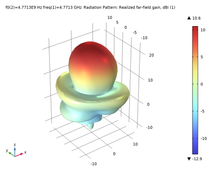
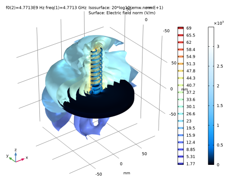
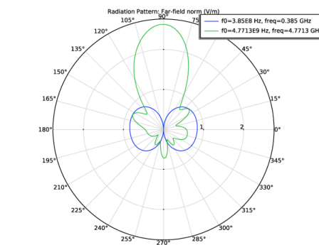
In the Model Builder window, expand the Results>2D Far Field (emw) node, then click Radiation Pattern 1.
2
In the Settings window for Radiation Pattern, locate the Evaluation section.
3
Find the Normal vector subsection. In the x text field, type 1.
4
In the z text field, type 0.
5
In the 2D Far Field (emw) toolbar, click  Plot.
As shown in Figure 4, the plotted pattern of the axial mode is more directive than that of the normal mode.
Radiation Pattern 1
1
Click the  Zoom Extents button in the Graphics toolbar.
Compare the reproduced axial mode 3D far-field pattern with that shown in Figure 5.
3D Far Field, Gain (emw)
1
In the Model Builder window, click 3D Far Field, Gain (emw).
2
In the Settings window for 3D Plot Group, locate the Data section.
3
From the Parameter value (f0 (Hz)) list, choose 3.85E8.
4
In the 3D Far Field, Gain (emw) toolbar, click  Plot.
5
Click the  Zoom Extents button in the Graphics toolbar.
See Figure 6 for the normal mode 3D far-field pattern.
S-parameter (emw)
The calculated S-parameters at the input port should be better than -10 dB for both modes.
3D Plot Group 6
1
In the Home toolbar, click  Add Plot Group and choose 3D Plot Group.
2
In the Settings window for 3D Plot Group, locate the Data section.
3
From the Dataset list, choose Study 1/Parametric Solutions 1 (sol2).
Isosurface 1
1
Right-click 3D Plot Group 6 and choose Isosurface.
2
In the Settings window for Isosurface, locate the Expression section.
3
In the Expression text field, type 20*log10(emw.normE+1).
4
Locate the Levels section. In the Total levels text field, type 20.
Filter 1
1
Right-click Isosurface 1 and choose Filter.
2
In the 3D Plot Group 6 toolbar, click  Plot.
3
In the Model Builder window, click Filter 1.
4
In the Settings window for Filter, locate the Element Selection section.
5
In the Logical expression for inclusion text field, type y>0.
6
In the 3D Plot Group 6 toolbar, click  Plot.
7
Click the  Zoom In button in the Graphics toolbar.
Surface 1
1
In the Model Builder window, right-click 3D Plot Group 6 and choose Surface.
2
In the Settings window for Surface, locate the Coloring and Style section.
3
Click  Change Color Table.
4
In the Color Table dialog box, select Aurora>JupiterAuroraBorealis in the tree.
5
Selection 1
1
Right-click Surface 1 and choose Selection.
2
You can do this most easily by copying the text ’13–49, 57, 58, 63, 64, 69, 70, and 72–105’ from the line above, clicking in the selection box, and then pressing Ctrl+V, or by using the Paste Selection dialog box.
3D Plot Group 6
1
In the Model Builder window, under Results click 3D Plot Group 6.
2
In the Settings window for 3D Plot Group, locate the Plot Settings section.
3
Clear the Plot dataset edges check box.
4
In the 3D Plot Group 6 toolbar, click  Plot.
Polar Plot Group 7
1
In the Home toolbar, click  Add Plot Group and choose Polar Plot Group.
2
In the Settings window for Polar Plot Group, locate the Data section.
3
From the Dataset list, choose Study 1/Parametric Solutions 1 (sol2).
4
From the Parameter selection (f0) list, choose From list.
5
In the Parameter values (f0 (Hz)) list, select 4.7713E9.
Radiation Pattern 1
1
In the Polar Plot Group 7 toolbar, click  More Plots and choose Radiation Pattern.
2
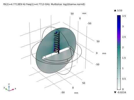
In the Settings window for Radiation Pattern, click Replace Expression in the upper-right corner of the Expression section. From the menu, choose Component 1 (comp1)>Electromagnetic Waves, Frequency Domain>Far field>emw.axialRatiodB - Axial ratio, dB.
3
Locate the Evaluation section. Find the Normal vector subsection. In the x text field, type 1.
4
In the z text field, type 0.
5
Find the Reference direction subsection. In the y text field, type 1.
6
In the x text field, type 0.
7
Find the Angles subsection. In the Number of angles text field, type 180.
8
Click to expand the Legends section. From the Legends list, choose Manual.
9
Select the Show legends check box.
10
11
Click to expand the Coloring and Style section. From the Width list, choose 2.
Polar Plot Group 7
1
In the Model Builder window, click Polar Plot Group 7.
2
In the Settings window for Polar Plot Group, locate the Axis section.
3
Select the Manual axis limits check box.
4
In the r minimum text field, type 0.
5
In the r maximum text field, type 10.
Radiation Pattern 2
1
In the Polar Plot Group 7 toolbar, click  More Plots and choose Radiation Pattern.
2
In the Settings window for Radiation Pattern, locate the Expression section.
3
In the Expression text field, type 3.
4
Locate the Evaluation section. Find the Normal vector subsection. In the x text field, type 1.
5
In the z text field, type 0.
6
Find the Reference direction subsection. In the y text field, type 1.
7
In the x text field, type 0.
8
Locate the Legends section. From the Legends list, choose Manual.
9
Select the Show legends check box.
10
11
Locate the Coloring and Style section. Find the Line style subsection. From the Line list, choose Dashed.
12
From the Color list, choose Red.
13
From the Width list, choose 2.
14
In the Polar Plot Group 7 toolbar, click  Plot.
Polar Plot Group 7
1
In the Model Builder window, click Polar Plot Group 7.
2
In the Settings window for Polar Plot Group, click to expand the Title section.
3
From the Title type list, choose Manual.
4
In the Title text area, type Axial ratio, dB.
5
In the Polar Plot Group 7 toolbar, click  Plot.
the axial ratio plot shows how much the antenna is circularly polarized. When it is characterized as the perfect circular polarization, the axial ratio is 1 or 0 dB. When it is below 3 dB (inside the red circle), it is typically regarded as a circular polarization. In the figure, the axial ratio is lower than 3 dB at the antenna boresight that is the major direction of propagation of the axial mode, parallel to the helical twist axis.