PDF

Fast Numerical Modeling of a Conical Horn Lens Antenna
Introduction
An axisymmetric 3D structure such as a conical horn antenna can be simulated in a fast and efficient way using only its 2D layout. In this example, the antenna radiation and matching characteristics are computed very quickly with respect to the dominant TE mode from the given circular waveguide by simulating the 2D axisymmetric geometry of an 3D antenna structure.
Figure 1: 3D model of the conical horn lens antenna from a 2D axisymmetric model.
Model Definition
The model consists of a conical metallic horn and a PTFE dielectric lens surrounded by an air domain. The outer part of the air domain truncated by perfectly matched layers (PML) that absorb the strong radiation from the horn aperture. All metal surfaces are assumed lossless, and so are modeled as perfect electric conductors (PEC). The lens material is also assumed lossless and configured as PTFE material with a low dielectric constant (εr = 2.1) to avoid unwanted sudden refractive index change between the air and the dielectric.
One end of the circular waveguide is excited with a predefined TE1 mode circular port boundary condition and the other end is connected to the conical horn, which is open to the air domain. The combination of azimuthal mode index and the circular port mode index in a 2D axisymmetric model is compatible with the predefined circular port mode index of a 3D model. The TE11 mode cutoff frequency of a circular waveguide with radius 10 mm is approximately 8.8 GHz, which is calculated by
where c0 is the speed of light, pnm are the roots of the derivative of the Bessel functions Jn(x), m and n are the mode indices, and a is the radius of a waveguide. The value of p11 is approximately 1.841. The operating frequency of the antenna is necessarily higher than the waveguide cutoff frequency.
The circular port boundary condition is placed on the interior boundary where the reflection and transmission characteristics are computed automatically in terms of S-parameters. The interior port boundary with PEC backing for one-way excitation requires the slit condition. The port orientation is specified to define the inward direction for the S-parameter calculation.
Results and Discussion
Figure 2 shows that the excited wave from the circular waveguide is traveling via the conical horn structure, confined via the dielectric lens, and generates a very directive radiation pattern. The radiation pattern is visualized in dB scale to get a better view of its sidelobes. The first sidelobe is about 22 dB lower than the main radiation lobe. The far-field radiation pattern in Figure 2 is just a simple body of revolution of the 2D plot data that is useful to measure quickly the maximum gain and review the overall shape of the pattern. The effective 3D far-field radiation pattern of the antenna excited by TE11 mode can be estimated using the predefined postprocessing function, normdB3DEfar_TE11(angle), that is shown in Figure 3.
Figure 2: 3D far-field radiation pattern in dB, visualized with the grid above the lens. The E-field norm is focused gradually toward the center.
 
Figure 3: Effective 3D far-field radiation pattern plotted in dB scale using far-far field function normdB3DEfar_TE11(angle).
Application Library path: RF_Module/Antennas/conical_horn_lens_antenna
Modeling Instructions
From the File menu, choose New.
New
In the New window, click  Model Wizard.
Model Wizard
1
In the Model Wizard window, click  2D Axisymmetric.
2
In the Select Physics tree, select Radio Frequency>Electromagnetic Waves, Frequency Domain (emw).
3
Click Add.
4
Click  Study.
5
In the Select Study tree, select General Studies>Frequency Domain.
6
Global Definitions
Parameters 1
1
In the Model Builder window, under Global Definitions click Parameters 1.
2
In the Settings window for Parameters, locate the Parameters section.
3
Click  Load from File.
4
First load the geometric parameters. Then calculate the cutoff frequency fc to ensure that a higher value is chosen for the simulation frequency f0.
5
Here, c_const is a predefined COMSOL constant for the speed of light in vacuum.
Study 1
Step 1: Frequency Domain
1
In the Model Builder window, under Study 1 click Step 1: Frequency Domain.
2
In the Settings window for Frequency Domain, locate the Study Settings section.
3
In the Frequencies text field, type f0.
Geometry 1
Circle 1 (c1)
1
In the Geometry toolbar, click  Circle.
2
In the Settings window for Circle, locate the Size and Shape section.
3
In the Radius text field, type hl*2.
4
In the Sector angle text field, type 180.
5
Locate the Position section. In the z text field, type 0.05.
6
Locate the Rotation Angle section. In the Rotation text field, type 270.
7
Click to expand the Layers section. In the table, enter the following settings:
8
Click  Build Selected.
Rectangle 1 (r1)
1
In the Geometry toolbar, click  Rectangle.
2
In the Settings window for Rectangle, locate the Size and Shape section.
3
In the Width text field, type r1.
4
In the Height text field, type wl.
5
Locate the Position section. In the z text field, type -wl.
Polygon 1 (pol1)
1
In the Geometry toolbar, click  Polygon.
2
In the Settings window for Polygon, locate the Coordinates section.
3
Polygon 2 (pol2)
1
In the Geometry toolbar, click  Polygon.
2
In the Settings window for Polygon, locate the Coordinates section.
3
Rectangle 2 (r2)
1
In the Geometry toolbar, click  Rectangle.
2
In the Settings window for Rectangle, locate the Size and Shape section.
3
In the Width text field, type ht.
4
In the Height text field, type wl.
5
Locate the Position section. In the r text field, type r1.
6
In the z text field, type -wl.
Parametric Curve 1 (pc1)
1
In the Geometry toolbar, click  More Primitives and choose Parametric Curve.
2
In the Settings window for Parametric Curve, locate the Parameter section.
3
In the Maximum text field, type max_para.
4
Locate the Expressions section. In the r text field, type s.
5
In the z text field, type -(s^2)*hlens/(max_para/1[m])^2.
6
Locate the Position section. In the z text field, type hl*cos(angle)+hlens+0.01.
Rectangle 3 (r3)
1
In the Geometry toolbar, click  Rectangle.
2
In the Settings window for Rectangle, locate the Size and Shape section.
3
In the Width text field, type max_para.
4
In the Height text field, type 0.01.
5
Locate the Position section. In the z text field, type hl*cos(angle).
6
In the Geometry toolbar, click  Build All.
Definitions
Perfectly Matched Layer 1 (pml1)
1
In the Definitions toolbar, click  Perfectly Matched Layer.
2
3
In the Settings window for Perfectly Matched Layer, locate the Geometry section.
4
In the Center coordinate text field, type 0.05.
Add Material
1
In the Home toolbar, click  Add Material to open the Add Material window.
2
Go to the Add Material window.
3
4
Click Add to Component in the window toolbar.
5
In the Home toolbar, click  Add Material to close the Add Material window.
Materials
Material 2 (mat2)
1
In the Model Builder window, under Component 1 (comp1) right-click Materials and choose Blank Material.
2
3
In the Settings window for Material, locate the Material Contents section.
4
Electromagnetic Waves, Frequency Domain (emw)
1
In the Model Builder window, under Component 1 (comp1) click Electromagnetic Waves, Frequency Domain (emw).
2
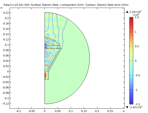
In the Settings window for Electromagnetic Waves, Frequency Domain, locate the Out-of-Plane Wave Number section.
3
In the m text field, type 1.
Perfect Electric Conductor 2
1
In the Physics toolbar, click  Boundaries and choose Perfect Electric Conductor.
2
Port 1
1
In the Physics toolbar, click  Boundaries and choose Port.
2
3
In the Settings window for Port, locate the Port Properties section.
4
From the Type of port list, choose Circular.
For the first port, wave excitation is on by default.
5
Select the Activate slit condition on interior port check box.
6
Click Toggle Power Flow Direction.
Far-Field Domain 1
In the Physics toolbar, click  Domains and choose Far-Field Domain.
Mesh 1
In the Home toolbar, click  Build Mesh.
Study 1
Step 1: Frequency Domain
Click  Compute.
Results
Electric Field (emw)
Visualize the model domains except for the perfectly matched layers.
Study 1/Solution 1 (sol1)
In the Model Builder window, expand the Results>Datasets node, then click Study 1/Solution 1 (sol1).
Selection
1
In the Results toolbar, click  Attributes and choose Selection.
2
In the Settings window for Selection, locate the Geometric Entity Selection section.
3
From the Geometric entity level list, choose Domain.
4
Surface
1
In the Model Builder window, expand the Electric Field (emw) node, then click Surface.
2
In the Settings window for Surface, locate the Expression section.
3
In the Expression text field, type emw.Er.
4
Click to expand the Range section. Select the Manual color range check box.
5
In the Minimum text field, type -1500.
6
In the Maximum text field, type 1500.
Contour 1
1
In the Model Builder window, right-click Electric Field (emw) and choose Contour.
2
In the Settings window for Contour, locate the Levels section.
3
In the Total levels text field, type 30.
4
Locate the Coloring and Style section. Clear the Color legend check box.
5
In the Electric Field (emw) toolbar, click  Plot.
The real parts of the Er and E-field norm contour shows that the wave is propagating toward the horn aperture and focused by the dielectric lens.
Radiation Pattern 1
Apply a finer angular resolution to get a better plot of the radiation pattern.
1
In the Model Builder window, expand the 2D Far Field (emw) node, then click Radiation Pattern 1.
2
In the Settings window for Radiation Pattern, locate the Evaluation section.
3
Find the Reference direction subsection. In the x text field, type -1.
4
In the z text field, type 0.
5
In the 2D Far Field (emw) toolbar, click  Plot.
3D Far Field, Gain (emw)
Add surface plots of the antenna body and lens, and show them together with the 3D far-field radiation pattern.
Radiation Pattern 1
1
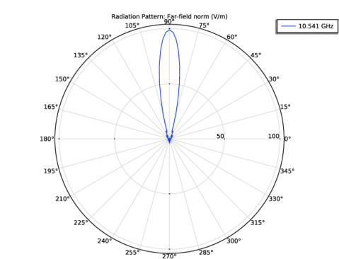
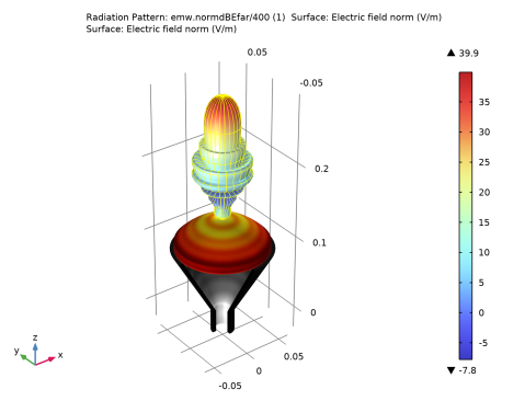
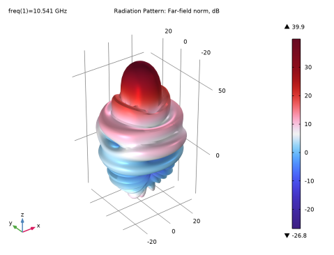
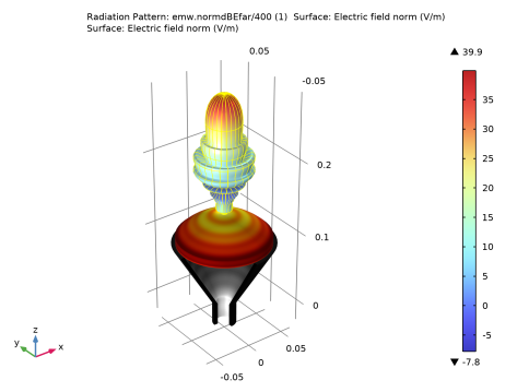
In the Model Builder window, expand the Results>3D Far Field, Gain (emw) node, then click Radiation Pattern 1.
2
In the Settings window for Radiation Pattern, click Replace Expression in the upper-right corner of the Expression section. From the menu, choose Component 1 (comp1)>Electromagnetic Waves, Frequency Domain>Far field>emw.normdBEfar - Far-field norm, dB - dB.
3
Locate the Expression section. In the Expression text field, type emw.normdBEfar/400.
This reduces the size of the 3D far-field radiation pattern.
4
Click Replace Expression in the upper-right corner of the Color section. From the menu, choose Component 1 (comp1)>Electromagnetic Waves, Frequency Domain>Far field>emw.normdBEfar - Far-field norm, dB - dB.
5
Locate the Evaluation section. Find the Angles subsection. In the Number of elevation angles text field, type 90.
6
Locate the Coloring and Style section. From the Grid list, choose Fine.
7
From the Color list, choose Yellow.
8
In the 3D Far Field, Gain (emw) toolbar, click  Plot.
9
Click the  Zoom Extents button in the Graphics toolbar.
Study 1/Solution 1 (2) (sol1)
In the Results toolbar, click  More Datasets and choose Solution.
Selection
1
In the Results toolbar, click  Attributes and choose Selection.
2
In the Settings window for Selection, locate the Geometric Entity Selection section.
3
From the Geometric entity level list, choose Domain.
4
Revolution 2D 2
1
In the Results toolbar, click  More Datasets and choose Revolution 2D.
2
In the Settings window for Revolution 2D, locate the Data section.
3
From the Dataset list, choose Study 1/Solution 1 (2) (sol1).
4
Click to expand the Revolution Layers section. In the Start angle text field, type -90.
5
In the Revolution angle text field, type 270.
Study 1/Solution 1 (3) (sol1)
In the Results toolbar, click  More Datasets and choose Solution.
Selection
1
In the Results toolbar, click  Attributes and choose Selection.
2
In the Settings window for Selection, locate the Geometric Entity Selection section.
3
From the Geometric entity level list, choose Domain.
4
Revolution 2D 3
1
In the Results toolbar, click  More Datasets and choose Revolution 2D.
2
In the Settings window for Revolution 2D, locate the Data section.
3
From the Dataset list, choose Study 1/Solution 1 (3) (sol1).
Surface 1
1
In the Model Builder window, right-click 3D Far Field, Gain (emw) and choose Surface.
2
In the Settings window for Surface, locate the Data section.
3
From the Dataset list, choose Revolution 2D 2.
4
Locate the Coloring and Style section. Click  Change Color Table.
5
In the Color Table dialog box, select Linear>GrayScale in the tree.
6
7
In the Settings window for Surface, locate the Coloring and Style section.
8
Clear the Color legend check box.
Surface 2
1
Right-click Surface 1 and choose Duplicate.
2
In the Settings window for Surface, locate the Data section.
3
From the Dataset list, choose Revolution 2D 3.
4
Locate the Coloring and Style section. Click  Change Color Table.
5
In the Color Table dialog box, select Thermal>ThermalDark in the tree.
6
7
In the 3D Far Field, Gain (emw) toolbar, click  Plot.
Deformation 1
1
In the Model Builder window, right-click Radiation Pattern 1 and choose Deformation.
2
In the Settings window for Deformation, locate the Expression section.
3
In the x-component text field, type 0.
4
In the y-component text field, type 0.
5
In the z-component text field, type 0.17.
6
Locate the Scale section.
7
Select the Scale factor check box. In the associated text field, type 1.
8
In the 3D Far Field, Gain (emw) toolbar, click  Plot.
9
Click the  Zoom Extents button in the Graphics toolbar.
This plot should reproduce Figure 2. The far-field radiation pattern plotted above is just a simple body of revolution of the 2D plot that is useful to measure quickly the maximum gain. Using the predefined postprocessing function, it is possible to estimate an effective 3D far-field radiation pattern of the antenna that is excited by the dominant mode of the 3D model of a circular waveguide, TE11 mode.
3D Plot Group 4
1
In the Home toolbar, click  Add Plot Group and choose 3D Plot Group.
2
In the Settings window for 3D Plot Group, locate the Data section.
3
From the Dataset list, choose None.
4
Locate the Color Legend section. Select the Show maximum and minimum values check box.
Radiation Pattern 1
1
In the 3D Plot Group 4 toolbar, click  More Plots and choose Radiation Pattern.
2
In the Settings window for Radiation Pattern, locate the Data section.
3
From the Dataset list, choose Study 1/Solution 1 (1) (sol1).
4
Locate the Expression section. In the Expression text field, type emw.normdB3DEfar_TE11(angle).
5
Locate the Evaluation section. Find the Angles subsection. In the Number of elevation angles text field, type 90.
6
In the Number of azimuth angles text field, type 90.
7
In the Azimuthal angle variable text field, type angle.
The far-field function contains an argument, which is given the name angle by default. For the azimuthal angle variable field in the Evaluation section, enter angle to match the function argument. Note that the name can be chosen freely as long as the function argument matches the azimuth angle variable specified in the Evaluation section.
8
Locate the Coloring and Style section. Click  Change Color Table.
9
In the Color Table dialog box, select Wave>Wave in the tree.
10
11
In the 3D Plot Group 4 toolbar, click  Plot.
Compare the plot with Figure 3.
12
Click the  Show More Options button in the Model Builder toolbar.
13
In the Show More Options dialog box, select Results>Plot Information Section in the tree.
14
In the tree, select the check box for the node Results>Plot Information Section.
15
When plotting a far-field radiation pattern, it may take a long time due to the finer resolution. The plotting time can be reviewed from the information section.
S-parameter (emw)
Finish by inspecting the S-parameter.