
 , and z are cylindrical coordinates centered on axis of the coaxial cable. Z is the wave impedance in the dielectric of the cable, and C is an arbitrary constant. The angular frequency is denoted by ω. The propagation constant, k, relates to the wavelength in the medium λ as
, and z are cylindrical coordinates centered on axis of the coaxial cable. Z is the wave impedance in the dielectric of the cable, and C is an arbitrary constant. The angular frequency is denoted by ω. The propagation constant, k, relates to the wavelength in the medium λ as
| 
                1	
               | 
| 
                2	
               | 
| 
                3	
               | Click Add. | 
| 
                4	
               | Click   Study. | 
| 
                5	
               | 
| 
                6	
               | Click   Done. | 
| 
                1	
               | 
| 
                2	
               | 
| 
                3	
               | Click   Browse. | 
| 
                4	
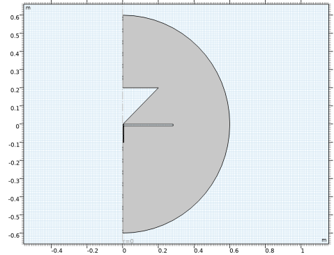
               | Browse to the model’s Application Libraries folder and double-click the file conical_antenna.mphbin. | 
| 
                5	
               | 
| 
                1	
               | 
| 
                2	
               | 
| 50 Ω | 
| 
                1	
               | 
| 
                2	
               | 
| 
                1	
               | 
| 
                2	
               | 
| 
                1	
               | 
| 
                2	
               | 
| 
                1	
               | 
| 
                2	
               | 
| 
                3	
               | 
| 
                1	
               | 
| 
                2	
               | 
| 
                3	
               | In the tree, select Built-in>Air. | 
| 
                4	
               | 
| 
                5	
               | 
| 
                1	
               | 
| 
                2	
               | 
| 
                1	
               | 
| 
                2	
               | 
| 
                3	
               | 
| 
                4	
               | 
| 
                1	
               | In the Model Builder window, under Component 1 (comp1) click Electromagnetic Waves, Frequency Domain (emw). | 
| 
                2	
               | 
| 
                3	
               | 
| 
                1	
               | 
| 
                3	
               | 
| 
                4	
               | 
| 
                1	
               | 
| 
                2	
               | 
| 
                3	
               | 
| 
                1	
               | 
| 
                1	
               | In the Model Builder window, expand the Far-Field Domain 1 node, then click Far-Field Calculation 1. | 
| 
                2	
               | 
| 
                3	
               | 
| 
                1	
               | 
| 
                2	
               | 
| 
                3	
               | 
| 
                4	
               | 
| 
                1	
               | 
| 
                2	
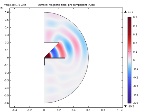
               | In the Settings window for Surface, click Replace Expression in the upper-right corner of the Expression section. From the menu, choose Component 1 (comp1)>Electromagnetic Waves, Frequency Domain>Magnetic>Magnetic field - A/m>emw.Hphi - Magnetic field, phi-component. | 
| 
                3	
               | 
| 
                4	
               | 
| 
                5	
               | 
| 
                6	
               | 
| 
                7	
               | 
| 
                8	
               | Click OK. | 
| 
                9	
               | 
| 
                10	
               | 
| 
                1	
               | 
| 
                2	
               | 
| 
                3	
               | 
| 
                4	
               | 
| 
                5	
               | 
| 
                6	
               | 
| 
                1	
               | 
| 
                2	
               | 
| 
                4	
               | Click to expand the Coloring and Style section. Find the Line style subsection. From the Line list, choose Cycle. | 
| 
                5	
               | 
| 
                1	
               | 
| 
                2	
               | 
| 
                3	
               | 
| 
                4	
               | 
| 
                1	
               | 
| 
                2	
               | 
| 
                3	
               | 
| 
                4	
               | Click Replace Expression in the upper-right corner of the r-Axis Data section. From the menu, choose Component 1 (comp1)>Electromagnetic Waves, Frequency Domain>Energy and power>emw.nPoav - Power outflow, time average - W/m². | 
| 
                5	
               | 
| 
                6	
               | 
| 
                7	
               | 
| 
                8	
               | 
| 
                9	
               | Click to expand the Coloring and Style section. Find the Line style subsection. From the Line list, choose Cycle. | 
| 
                10	
               | Click to collapse the Coloring and Style section. Click to expand the Legends section. Select the Show legends check box. | 
| 
                11	
               | 
| 
                13	
               | 
| 
                14	
               | 
| 
                1	
               | 
| 
                2	
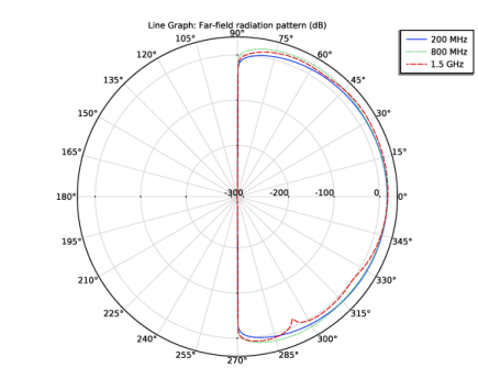
               | In the Settings window for Line Graph, click Replace Expression in the upper-right corner of the r-Axis Data section. From the menu, choose Component 1 (comp1)>Electromagnetic Waves, Frequency Domain>Far field>emw.normdBEfar - Far-field norm, dB - dB. | 
| 
                3	
               | 
| 
                4	
               |