PDF

Axisymmetric Cavity Resonator
Introduction
In this example, the resonant frequencies and fields of an axisymmetric cavity are obtained using the 2D axisymmetric formulation that is available with either the RF Module or the Wave Optics Module. The cross section of the cavity is rectangular and the walls are perfect electric conductors (PEC). For this geometry, applying separation of variables results in transcendental equations for the eigenfrequencies, and so this example serves as a benchmark for the 2D axisymmetric formulation. The resonant frequencies obtained with COMSOL Multiphysics agree with the solutions of the transcendental equations to 1 part in 106, which is the default tolerance of the eigenvalue solver. The model also demonstrates that the solutions obtained using the 2D axisymmetric formulation can be rotated rotate about the z-axis to obtain a 3D solution.
Model Definition
The cavity is axisymmetric with a rectangular cross section as shown in Figure 1. The cavity walls are PEC and the region of interest is the interior of the cavity, which is vacuum.
Figure 1: Geometry of the resonant cavity. From left to right: full view, 3/4 cut-away view, cross section in the rz-plane.
The problem is solved in the frequency domain. The assumed time dependence is ejωt, where ω is the angular frequency and is related to the frequency f by ω = 2πf. The time-harmonic form of the curl-curl equation is a homogeneous eigenvalue equation in the electric field E and the unknown eigenvalue ω2, shown below.
(1)
Since the material properties and the geometry are axisymmetric, the model can be solved with the 2D axisymmetric formulation. The computational domain is the rz-plane and the dependent variables are the cylindrical components of the electric field Er(r, z), Eφ(r, z), and Ez(r, z), which are, in general, complex.
The angular dependence of the field is assumed to be of the form , where m is an integer called the azimuthal mode number. The azimuthal mode number is specified by the user. The eigenfrequencies for the resonant cavity will be solved for 01, and 2 using a parametric sweep, which is similar to a for loop.
The combined temporal and angular dependence of the field components is . The physical quantities are obtained from the dependent variables using the expressions below, where Re{…} indicates the real part of the complex quantity.
(2)
(3)
(4)
Suppose that Ez(r, z) is purely real, in which case the preceding equation reduces to
(5).
For m > 0, the field rotates in the + direction and for m < 0, the field rotates in the  direction. This is also true if Ez(r, z) is complex and it also holds for the other field components. This is shown explicitly in the animation at the end of the example.
Results and Discussion
The default plot is the norm of the electric field. This plot can be used as a diagnostic tool to determine whether a particular mode is physical or spurious. The lowest-frequency physical modes have spatial variation that is comparable to the size of the cavity, while the spurious modes have a spatial variation that is comparable to the mesh size. The norm of the electric field is plotted for 4 of the lowest-frequency (physical) modes below in Figure 2 to Figure 5.
An arrow plot of the electric field for the = 1 mode at 2.122059 GHz is shown in Figure 6. This plot is animated at the end of the example.
Figure 2: Norm of the electric field for the m=0 mode at 1.499 GHz.
Figure 3: Norm of the electric field for the m=1 mode at 1.692 GHz.
Figure 4: Norm of the electric field for the m=1 mode at 2.122 GHz.
Figure 5: Norm of the electric field for the m=2 mode at 2.076 GHz.
Figure 6: An arrow plot of the electric field for the m=1 mode at 2.122 GHz.
An analytical solution to this problem can be obtained using separation of variables. Details of the derivation can be found in Ref. 1. There is a transcendental equation involving Bessel functions for the eigenvalue k2 = ω2/c2. The values for 8 modes are contained in the left column of the table below. The right column contains the values obtained using COMSOL Multiphysics. The results agree to 1 part in 106, which is the default tolerance of the eigenvalue solver.
References
1. C.M. Pinciuc, Basis Functions With Divergence Constraints For The Finite Element Method, Ph.D. thesis, Dept. Electrical and Computer Eng., Univ. of Toronto, 2012, Appendix C, pp. 174–181.
2. J.D. Jackson, Classical Electrodynamics, 3rd Edition, John Wiley & Sons, 1999, p. 399 (Problem 8.7).
Application Library path: RF_Module/Verification_Examples/axisymmetric_cavity_resonator
Modeling Instructions
From the File menu, choose New.
New
In the New window, click  Model Wizard.
Model Wizard
1
In the Model Wizard window, click  2D Axisymmetric.
2
In the Select Physics tree, select Radio Frequency>Electromagnetic Waves, Frequency Domain (emw).
3
Click Add.
4
Click  Study.
5
In the Select Study tree, select General Studies>Eigenfrequency.
6
Global Definitions
Parameters 1
1
In the Model Builder window, under Global Definitions click Parameters 1.
2
In the Settings window for Parameters, locate the Parameters section.
3
Geometry 1
Create a rectangle for the 2D axisymmetric geometry.
Rectangle 1 (r1)
1
In the Geometry toolbar, click  Rectangle.
2
In the Settings window for Rectangle, locate the Size and Shape section.
3
In the Width text field, type b-a.
4
In the Height text field, type height.
5
Locate the Position section. In the r text field, type a.
6
In the Geometry toolbar, click  Build All.
The completed geometry should look the same as in the figure that follows.
Materials
Assign material properties of the vacuum to the interior of the cavity.
Vacuum
1
In the Model Builder window, under Component 1 (comp1) right-click Materials and choose Blank Material.
2
In the Settings window for Material, type Vacuum in the Label text field.
3
Locate the Material Contents section. In the table, enter the following settings:
Electromagnetic Waves, Frequency Domain (emw)
Change the azimuthal mode number to the parameter defined in the table above.
1
In the Model Builder window, under Component 1 (comp1) click Electromagnetic Waves, Frequency Domain (emw).
2
In the Settings window for Electromagnetic Waves, Frequency Domain, locate the Out-of-Plane Wave Number section.
3
In the m text field, type m_azimuthal.
Mesh 1
1
In the Model Builder window, under Component 1 (comp1) click Mesh 1.
2
In the Settings window for Mesh, locate the Physics-Controlled Mesh section.
3
In the table, clear the Use check box for Electromagnetic Waves, Frequency Domain (emw).
For electromagnetic wave problems, the maximum mesh size should be smaller than 1/5 of the wavelength. The spatial variation of the lowest frequency resonant modes is comparable to the cavity size, so the default mesh is a reasonable starting point. This will turn out to be very accurate for this simple model. However, in a general case where the exact solutions are not known, a mesh refinement analysis is useful.
4
In the Home toolbar, click  Build Mesh.
Study 1
Solve for 12 cavity modes near 2 GHz, an estimate for the lowest resonant frequency based on the size of the cavity. A reasonable value is necessary so that not all of the solutions are spurious modes.
Step 1: Eigenfrequency
1
In the Model Builder window, under Study 1 click Step 1: Eigenfrequency.
2
In the Settings window for Eigenfrequency, locate the Study Settings section.
3
Select the Desired number of eigenfrequencies check box. In the associated text field, type 12.
4
In the Search for eigenfrequencies around text field, type 2[GHz].
Perform a parametric sweep over the azimuthal mode number, which is similar to a for loop.
Parametric Sweep
1
In the Study toolbar, click  Parametric Sweep.
2
In the Settings window for Parametric Sweep, locate the Study Settings section.
3
4
5
In the Study toolbar, click  Compute.
Results
Look at plots of the norm of the electric field. The smoothly varying solutions are physical modes. The spatial variation of the field is comparable to the cavity size. The spurious modes have spatial variation comparable to the mesh size. In fact, the resonant frequency and fields of the spurious modes are extremely mesh-dependent. From the plots, it is possible to determine that the lowest frequency resonant mode is approximately 1.49896 GHz.
Electric Field (emw)
1
In the Model Builder window, under Results click Electric Field (emw).
2
In the Settings window for 2D Plot Group, locate the Data section.
3
From the Parameter value (m_azimuthal) list, choose 0.
4
From the Eigenfrequency (GHz) list, choose 1.499.
5
In the Electric Field (emw) toolbar, click  Plot.
This plot should look like Figure 2 above. The other 2D plots can be produced following the instructions below.
6
From the Parameter value (m_azimuthal) list, choose 1.
7
From the Eigenfrequency (GHz) list, choose 3.0989.
8
In the Electric Field (emw) toolbar, click  Plot.
9
From the Eigenfrequency (GHz) list, choose 3.673.
10
In the Electric Field (emw) toolbar, click  Plot.
11
From the Parameter value (m_azimuthal) list, choose 2.
12
From the Eigenfrequency (GHz) list, choose 4.2648.
13
In the Electric Field (emw) toolbar, click  Plot.
Evaluate k2 to compare with the solutions obtained via separation of variables. The conditional statement that appears in the expression ensures that there are nonzero values for the physical modes only, that is, the expression evaluates to zero for the spurious modes.
Global Evaluation 2
1
In the Results toolbar, click  Global Evaluation.
2
In the Settings window for Global Evaluation, locate the Data section.
3
From the Dataset list, choose Study 1/Parametric Solutions 1 (sol2).
4
From the Table columns list, choose Outer solutions.
5
Locate the Expressions section. In the table, enter the following settings:
6
Click  Evaluate.
Revolution 2D
After computing the solution to the 2D axisymmetric problem, a revolution of the 2D dataset is produced. The revolved dataset can be used in 3D plots. Set the start angle to 0 and the revolution angle to 360.
1
In the Model Builder window, expand the Results>Datasets node, then click Revolution 2D.
2
In the Settings window for Revolution 2D, click to expand the Revolution Layers section.
3
In the Start angle text field, type 0.
4
In the Revolution angle text field, type 360.
5
Click to expand the Advanced section. Select the Define variables check box.
The last step defines a variable for the angle, rev1phi, which can be used in a 3D arrow plot of the electric field.
3D Plot Group 2
In the Results toolbar, click  3D Plot Group.
Arrow Volume 1
1
In the 3D Plot Group 2 toolbar, click  Arrow Volume.
2
In the Settings window for Arrow Volume, locate the Expression section.
3
In the R-component text field, type Er*exp(-i*m_azimuthal*rev1phi).
4
In the PHI-component text field, type Ephi*exp(-i*m_azimuthal*rev1phi).
5
In the Z-component text field, type Ez*exp(-i*m_azimuthal*rev1phi).
6
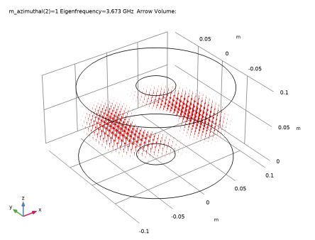
Locate the Arrow Positioning section. Find the X grid points subsection. In the Points text field, type 30.
7
Find the Y grid points subsection. In the Points text field, type 30.
8
Find the Z grid points subsection. In the Points text field, type 1.
9
In the 3D Plot Group 2 toolbar, click  Plot.
3D Electric Field
1
In the Model Builder window, under Results click 3D Plot Group 2.
2
In the Settings window for 3D Plot Group, type 3D Electric Field in the Label text field.
3
Locate the Data section. From the Parameter value (m_azimuthal) list, choose 1.
4
From the Eigenfrequency (GHz) list, choose 3.673.
5
In the 3D Electric Field toolbar, click  Plot.
This plot should look like Figure 6 above. Now convert the plot into a movie. Note that to make a frequency domain dataset oscillate in time, the sequence type is set to dynamic data extension.
Animation 1
1
In the Results toolbar, click  Animation and choose File.
2
In the Settings window for Animation, locate the Target section.
3
From the Target list, choose Player.
4
Locate the Scene section. From the Subject list, choose 3D Electric Field.
5
Locate the Animation Editing section. From the Sequence type list, choose Dynamic data extension.
6
Click the  Play button in the Graphics toolbar.