Free Convection in a Porous Medium

This example describes flow in porous media driven by density variations that result from temperature changes. The example comes from Hossain and Wilson (Ref. 1), who use a specialized in-house code to solve this free-convection problem. This COMSOL Multiphysics example reproduces their work using the Brinkman Equations interface and the Heat Transfer in Porous Media interface. The results of this model match those of the published study.

Model Definition

The following figure gives the example geometry. Water in a porous medium layer can move within the layer but not exit from it. Temperatures vary from high to low along the outer edges. Initially the water is stagnant, but temperature gradients alter the fluid density to the degree that buoyant flow occurs. The problem statement specifies that the flow is steady state.

Figure 1: Domain geometry and boundary conditions for the heat balance in the free-convection problem. Th is a higher temperature than Tc, while s is a variable that represents the relative length of a boundary segment and goes from 0 to 1 along the segment.

Model this free-convection problem by introducing a Boussinesq buoyancy term to Brinkman’s momentum equation, and then linking the resulting fluid velocities to the Heat Transfer in Porous Media interface.

The Boussinesq buoyancy term that appears on the right-hand side of the momentum equation accounts for the lifting force due to thermal expansion

(1)

In these expressions, T represents temperature, while Tc is a reference temperature, g denotes the gravity acceleration, ρ gives the fluid density at the reference temperature, ε is the porosity, and αp is the fluid’s coefficient of volumetric thermal expansion.

The heat balance comes from the heat transfer equation

(2)

where keq denotes the effective thermal conductivity of the fluid-solid mixture, and CL is the fluid’s heat capacity at constant pressure.

The boundary conditions for the Brinkman equations are all no-slip conditions. Using only velocity boundaries gives no information on the pressure within the domain, which means that the example produces estimates of the pressure change instead of the pressure field. However, without any seed information on pressure, the problem is unlikely to converge. The remedy is to arbitrarily fix the pressure at a point in the example using a point constraint. The boundary conditions for the Heat Transfer interface are the series of fixed temperatures shown in Figure 1.

Implementation: Initial Conditions for Boussinesq Approximation

The simple statements in Equation 1 and Equation 2 produce a strong nonlinear problem that represents a difficult convergence task for most nonlinear solvers. To ease the numerical difficulties, let the coefficient of volumetric thermal expansion αp increase gradually, raising the Rayleigh number of the experiment. When αp = 0, the momentum and temperature equations are uncoupled, so the example converges easily. Then increase αp, using the previous solution as the initial guess for the next parametric step, and so on, until reaching a Rayleigh number of 105. The iteration protocol is an easy process with the parametric solver in COMSOL Multiphysics.

Results

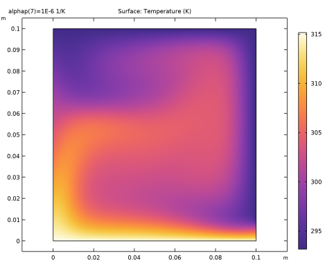
This example reproduces a model reported by Hossain and Wilson (Ref. 1). After extracting the input data from the paper, the author constructed the example in less than an hour, including all the steps from geometry input to postprocessing of the results. Figure 2 shows the temperature distribution throughout the porous slice.

Figure 2: Temperature in a porous structure subjected to temperature gradients and subsequent free convection. The COMSOL Multiphysics simulation is in excellent agreement with published results from Ref. 1.

Figure 3 gives the COMSOL Multiphysics solution for the flow field.

Figure 3: Velocity field for a Rayleigh number of Ra = 105.

Reference

1. M. Anwar Hossain and M. Wilson, “Natural Convection Flow in a Fluid-saturated Porous Medium Enclosed by Non-isothermal Walls with Heat Generation,” Int. J. Therm. Sci., vol. 41, pp. 447–454, 2002.

Porous_Media_Flow_Module/Heat_Transfer/convection_porous_medium

Modeling Instructions

From the menu, choose .

New

In the window, click

Model Wizard

In the window, click

In the tree, select .

Click .

Click

In the tree, select .

Click

Global Definitions

Parameters 1

Start by loading parameters from a file. The list contains material parameters and also parameters for setting up the physics.

In the window, under click .

In the window for , locate the section.

Click

Browse to the model’s Application Libraries folder and double-click the file convection_porous_medium_parameters.txt.

Geometry 1

Square 1 (sq1)

In the toolbar, click

In the window for , locate the section.

In the text field, type L.

Point 1 (pt1)

In the toolbar, click

In the window for , locate the section.

In the text field, type L.

In the text field, type L/10.

Click

Materials

With choosing the Nonisothermal Flow, Brinkman Equations multiphysics interface a is added automatically.

Porous Material 1 (pmat1)

In the window, expand the node, then click .

In the window for , locate the section.

In the table, enter the following settings:


Property	Variable	Value	Unit	Property group
Permeability	kappa_iso ; kappaii = kappa_iso, kappaij = 0	kappa	m²	Basic

Fluid (pmat1.fluid)

In the window, expand the node, then click .

In the window for , locate the section.

In the table, enter the following settings:


Property	Variable	Value	Unit	Property group
Density	rho	rho0	kg/m³	Basic
Heat capacity at constant pressure	Cp	Cp0	J/(kg·K)	Basic
Thermal conductivity	k_iso ; kii = k_iso, kij = 0	k0	W/(m·K)	Basic
Dynamic viscosity	mu	mu0	Pa·s	Basic

Solid (pmat1.solid)

In the window, click .

In the window for , locate the section.

In the θs text field, type 1-epsilon.

Locate the section. In the table, enter the following settings:


Property	Variable	Value	Unit	Property group
Density	rho	0	kg/m³	Basic
Heat capacity at constant pressure	Cp	0	J/(kg·K)	Basic
Thermal conductivity	k_iso ; kii = k_iso, kij = 0	0	W/(m·K)	Basic