PDF

Flow of Viscoelastic Fluid Past a Cylinder
Introduction
Many complex fluids of interest exhibit a combination of viscous and elastic behavior under strain. Examples of such fluids are polymer solutions and melts, oil, toothpaste, and clay, among many others. The Oldroyd-B fluid presents one of the simplest constitutive models capable of describing the viscoelastic behavior of dilute polymeric solutions under general flow conditions. Despite the apparent simplicity of the constitutive relation, the dynamics that arise in many flows are complicated enough to present a considerable challenge to numerical simulations.
Model Definition
This example studies a flow of Oldroyd-B fluid past a cylinder between two parallel plates. The flow is considered as being two-dimensional (2D). The aspect ratio of the cylinder radius to the to the channel half-width is 1/2.
The fluid is a dilute solution of polymer in a Newtonian liquid solvent of viscosity μs. The total stress is presented as
where u = (uv) is the flow velocity vector, p is the pressure, and
is the strain rate. The extra stress contribution due to the polymer is given by the following Oldroyd-B constitutive relation:
(1)
where the upper convective derivative operator is defined as
The polymer is characterized by two physical parameters: the viscosity μp and the relaxation time λ.
Nondimensional Formulation
The Weissenberg number is defined as:
where Uin is the average fluid velocity at the inlet, R is the radius of the cylinder, and λ is the polymer relaxation time.
A zero Weissenberg number gives a pure viscous fluid (no elasticity), while the infinite Weissenberg number limit corresponds to purely elastic response. Due to the convective nature of the constitutive relation, solution stability is lost with increasing fluid elasticity. In practice, already values Wi > 1 are considered as a high for many flows of an Oldroyd-B fluid.
The flow is stationary, and the problem becomes dimensionless by using R, Uin, and the total viscosity μ = μs + μp. The Reynolds number is defined as
(2)
Boundary Conditions
Because of the flow symmetry, it is sufficient to model only the upper halves of the channel and the cylinder. At the channel centerline, use the symmetry conditions of zero normal flow and zero total tangential stress. At the channel walls and the cylinder surface, the model uses no slip boundary conditions. At the inlet, the fully developed parabolic velocity profile and the corresponding extra stresses components are specified:
At the outlet, use the pressure boundary condition for developed flow; the only stress acting at the boundary is due to the pressure force pout:
Results
The analysis gradually increases the Weissenberg number from 0 to 1 using the parametric solver. Figure 1 and Figure 2 show the flow field and stress distribution for the value Wi = 0.7. Figure 3 shows the drag coefficient as a function of the Weissenberg number. The result is in good agreement with the experimental and simulation results presented in Ref. 2.
Figure 1: Flow field near cylinder and stress distribution for Wi = 0.7.
Figure 2: Stress distribution along the cylinder surface and wake centerline for Wi = 0.7.
Figure 3: Drag on the cylinder.
References
1. T.J. Craven, J.M. Rees, and W.B. Zimmerman, “Stabilized finite element modelling of Oldroyd-B viscoelastic flow,” COMSOL Conference 2006, Birmingham, U.K., 2006.
2. M.A. Alves, F.T. Pinho, and P.J. Oliveira, “The flow of viscoelastic fluids past a cylinder: finite-volume high-resolution methods,” J. Non-Newtonian Fluid Mech., vol. 97, pp. 207–232, 2001.
Application Library path: Polymer_Flow_Module/Verification_Examples/cylinder_flow_viscoelastic
Modeling Instructions
From the File menu, choose New.
New
In the New window, click  Model Wizard.
Model Wizard
1
In the Model Wizard window, click  2D.
2
In the Select Physics tree, select Fluid Flow>Single-Phase Flow>Viscoelastic Flow (vef).
3
Click Add.
4
Click  Study.
5
In the Select Study tree, select General Studies>Stationary.
6
Root
1
In the Model Builder window, click the root node.
2
In the root node’s Settings window, locate the Unit System section.
3
From the Unit system list, choose None.
The equations you will solve are formulated in dimensionless form.
Geometry 1
Rectangle 1 (r1)
1
In the Geometry toolbar, click  Rectangle.
2
In the Settings window for Rectangle, locate the Size and Shape section.
3
In the Width text field, type 25.
4
In the Height text field, type 2.
5
Locate the Position section. In the x text field, type -10.
6
Click  Build Selected.
Rectangle 2 (r2)
1
In the Geometry toolbar, click  Rectangle.
2
In the Settings window for Rectangle, locate the Size and Shape section.
3
In the Width text field, type 6.
4
In the Height text field, type 2.
5
Locate the Position section. In the x text field, type -2.
6
Click  Build Selected.
Circle 1 (c1)
1
In the Geometry toolbar, click  Circle.
2
In the Settings window for Circle, click  Build Selected.
Difference 1 (dif1)
1
In the Geometry toolbar, click  Booleans and Partitions and choose Difference.
2
Select the objects r1 and r2 only.
3
In the Settings window for Difference, locate the Difference section.
4
Find the Objects to subtract subsection. Click to select the  Activate Selection toggle button.
5
6
Click  Build Selected.
Global Definitions
Parameters 1
1
In the Model Builder window, under Global Definitions click Parameters 1.
2
In the Settings window for Parameters, locate the Parameters section.
3
Viscoelastic Flow (vef)
Fluid Properties 1
1
In the Model Builder window, under Component 1 (comp1)>Viscoelastic Flow (vef) click Fluid Properties 1.
2
In the Settings window for Fluid Properties, locate the Fluid Properties section.
3
From the ρ list, choose User defined. In the associated text field, type Re.
4
Find the Constitutive relation subsection. From the μs list, choose User defined. In the associated text field, type mu_s.
5
Inlet 1
1
In the Physics toolbar, click  Boundaries and choose Inlet.
2
3
In the Settings window for Inlet, locate the Velocity section.
4
Click the Velocity field button.
5
Specify the u0 vector as
6
Locate the Viscoelastic Stress section. From the list, choose Symmetric.
7
In the Te0 table, enter the following settings:
Outlet 1
1
In the Physics toolbar, click  Boundaries and choose Outlet.
2
3
In the Settings window for Outlet, locate the Pressure Conditions section.
4
Clear the Suppress backflow check box.
Symmetry 1
1
In the Physics toolbar, click  Boundaries and choose Symmetry.
2
Click the  Zoom Extents button in the Graphics toolbar.
3
Proceed to set up boundary probe to compute the drag coefficient.
Definitions
Boundary Probe 1 (bnd1)
1
In the Definitions toolbar, click  Probes and choose Boundary Probe.
2
In the Settings window for Boundary Probe, locate the Probe Type section.
3
From the Type list, choose Integral.
4
Locate the Source Selection section. Click  Clear Selection.
5
6
In the Variable name text field, type Cd.
7
Locate the Expression section. In the Expression text field, type -2*(vef.T_stressx).
8
Select the Description check box. In the associated text field, type Cd.
Mesh 1
Size
In the Model Builder window, under Component 1 (comp1) right-click Mesh 1 and choose Edit Physics-Induced Sequence.
Size 1
1
2
In the Settings window for Size, locate the Element Size section.
3
From the Predefined list, choose Extra fine.
4
Click  Build Selected.
Mapped 1
1
In the Mesh toolbar, click  Mapped.
2
In the Settings window for Mapped, locate the Domain Selection section.
3
From the Geometric entity level list, choose Domain.
4
Distribution 1
1
Right-click Mapped 1 and choose Distribution.
2
3
In the Settings window for Distribution, locate the Distribution section.
4
From the Distribution type list, choose Predefined.
5
In the Number of elements text field, type 20.
6
In the Element ratio text field, type 5.
7
Click  Build Selected.
Distribution 2
1
In the Model Builder window, right-click Mapped 1 and choose Distribution.
2
3
In the Settings window for Distribution, locate the Distribution section.
4
From the Distribution type list, choose Predefined.
5
In the Number of elements text field, type 25.
6
In the Element ratio text field, type 5.
7
Select the Reverse direction check box.
8
Click  Build All.
Study 1
Step 1: Stationary
1
In the Model Builder window, under Study 1 click Step 1: Stationary.
2
In the Settings window for Stationary, click to expand the Study Extensions section.
3
Select the Auxiliary sweep check box.
4
5
From the list in the Parameter name column, choose Wi (Weissenberg number).
6
Click  Range.
7
In the Range dialog box, type 0 in the Start text field.
8
In the Stop text field, type 1.
9
In the Step text field, type 0.05.
10
Click Replace.
11
In the Settings window for Stationary, locate the Study Extensions section.
12
From the Run continuation for list, choose No parameter.
13
From the Reuse solution from previous step list, choose Yes.
14
In the Home toolbar, click  Compute.
Results
Velocity (vef)
To monitor the variation of the drag on the cylinder due to the flow, click on the Probe Plot tab once it becomes available.
Once the solution is complete, the plot of the flow field appears. Adjust the view to magnify the region around the cylinder, then add a contour plot for the extra stresses. Follow these steps:
Definitions
View 1
1
In the Model Builder window, under Component 1 (comp1)>Definitions click View 1.
2
In the Settings window for View, locate the View section.
3
Select the Lock axis check box.
Axis
1
In the Model Builder window, expand the View 1 node, then click Axis.
2
In the Settings window for Axis, locate the Axis section.
3
In the x minimum text field, type -2.
4
In the x maximum text field, type 6.
5
In the y minimum text field, type -4.
6
In the y maximum text field, type 4.
Results
Velocity (vef)
1
In the Model Builder window, under Results click Velocity (vef).
2
In the Settings window for 2D Plot Group, locate the Plot Settings section.
3
From the View list, choose View 1.
4
Locate the Data section. From the Parameter value (Wi) list, choose 0.7.
5
Locate the Plot Settings section. Clear the Plot dataset edges check box.
Contour 1
1
Right-click Velocity (vef) and choose Contour.
2
In the Settings window for Contour, click Replace Expression in the upper-right corner of the Expression section. From the menu, choose Component 1 (comp1)>Viscoelastic Flow>Viscoelastic variables>Viscoelastic extra stress tensor, branch 1>vef.Te_1xx - Viscoelastic extra stress tensor, branch 1, xx-component.
3
Locate the Levels section. In the Total levels text field, type 40.
4
Locate the Coloring and Style section. Click  Change Color Table.
5
In the Color Table dialog box, select Linear>GrayScale in the tree.
6
7
In the Velocity (vef) toolbar, click  Plot.
You should now obtain the plot shown in Figure 1.
To plot the stress variation along the cylinder surface and in the wake, follow these steps:
1D Plot Group 4
In the Home toolbar, click  Add Plot Group and choose 1D Plot Group.
Line Graph 1
1
Right-click 1D Plot Group 4 and choose Line Graph.
2
3
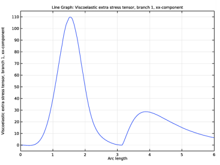
In the Settings window for Line Graph, click Replace Expression in the upper-right corner of the y-Axis Data section. From the menu, choose Component 1 (comp1)>Viscoelastic Flow>Viscoelastic variables>Viscoelastic extra stress tensor, branch 1>vef.Te_1xx - Viscoelastic extra stress tensor, branch 1, xx-component.
4
In the 1D Plot Group 4 toolbar, click  Plot.
1D Plot Group 4
1
In the Model Builder window, click 1D Plot Group 4.
2
In the Settings window for 1D Plot Group, locate the Data section.
3
From the Parameter selection (Wi) list, choose From list.
4
In the Parameter values (Wi) list, select 0.7.
5
Locate the Axis section. Select the Manual axis limits check box.
6
In the x minimum text field, type 0.
7
In the x maximum text field, type 6.
8
In the y minimum text field, type -5.
9
In the y maximum text field, type 115.
10
In the 1D Plot Group 4 toolbar, click  Plot.
This will produce the stress plot shown in Figure 2.
Finally, check the complete probe plot of the drag coefficient and compare it to that shown in Figure 3.
Drag coefficient
1
In the Model Builder window, under Results click Probe Plot Group 3.
2
In the Settings window for 1D Plot Group, type Drag coefficient in the Label text field.