PDF

Plasma DC Arc
Introduction
Thermal plasmas have nowadays a large range of industrial applications including cutting, welding, spraying, waste destruction, and surface treatment. Thermal plasmas are assumed to be under partial to complete local thermodynamic equilibrium (LTE) conditions. Under LTE, the plasma can be considered a conductive fluid mixture and therefore be modeled using the magnetohydrodynamics (MHD) equations. This model shows how to use the Equilibrium Discharges, In-Plane Currents interface (available in 2D and 2D axisymmetric) interface to simulate the plasma generated in a DC arc.
Note: This application requires the Plasma Module and AC/DC Module.
Model Definition
This model is based on the work presented in Ref. 1. In Ref. 1, the authors develop a complex model that includes the description of the weld pool under the action of a pulsed arc. In this work, only the plasma and the transfer of heat and currents in the metals are simulated, neglecting the weld pool, and a DC excitation is used. These simplifications make it possible to have a model that solves fast, that can be used to understand basic physical effects, and that can be used as initial conditions for a time-dependent model.
The model is solved using a stationary study. A current of 80 A is set at the cathode and the bottom plate is grounded. In the 5 mm gap between the electrodes, an argon plasma arc is created that heats the metal electrodes and surrounding gas. A shielding flow is added along the cathode.
The temperature-dependent physical properties of argon are loaded from the material library under Equilibrium Discharge. The temperature range of the physical properties span from 500 K to 25,000 K. A minimum electrical conductivity of 1 S/m is used for numerical stability reasons. Another important aspect to keep in mind is that the model used is not valid to describe the plasma sheath region since in this regions there is charge separation and deviations from equilibrium. From the practical point of view, having a fine resolution in the plasma-electrode region causes numerical instabilities (and does not bring a better description of the physics). To make the model more stable, use a mesh that is coarse enough so that the plasma sheath is averaged out.
In this model, the initial condition need special attention. It is very difficult to start from a flat profile of temperature. It is necessary to add an initial high temperature region between the electrodes.
Results and Discussion
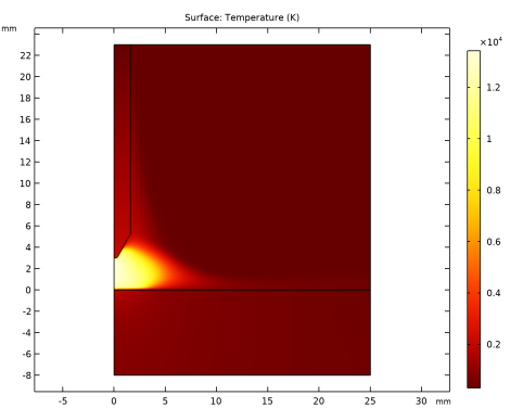
Figure 1, Figure 2, and Figure 3 show the temperatures in the solids and gas, fluid velocity, and electrical conductivity. The temperature reaches a maximum of 14,000 K at the anode region. The fluid velocity in the electrodes gap is much larger that the inlet as a consequence of the pressure and Lorentz forces. Note also that the conductivity in the gap is of the order or 10k S/m, thus creating an effective conducting channel.
Figure 1: Plot of the LTE plasma temperature.
Figure 2: Plot of the velocity magnitude of the fluid.
Figure 3: Plot of the electrical conductivity.
Reference
1. A. Traidia, F. Roger, A. Chidley, J. Schroeder, and T. Marlaud “Effect of Helium-Argon Mixtures on the Heat Transfer and Fluid Flow in Gas Tungsten Arc Welding,” Int. J. Mech. Mechatron., vol. 5, no. 1, pp. 223–228, 2011.
Application Library path: Plasma_Module/Equilibrium_Discharges/plasma_dc_arc
Modeling Instructions
From the File menu, choose New.
New
In the New window, click  Model Wizard.
Model Wizard
1
In the Model Wizard window, click  2D Axisymmetric.
2
In the Select Physics tree, select Plasma>Equilibrium Discharges>Equilibrium Discharges, In-Plane Currents.
3
Click Add.
4
Click  Study.
5
In the Select Study tree, select General Studies>Stationary.
6
Geometry 1
Select the mm units and create the geometry for the arc model.
1
In the Model Builder window, under Component 1 (comp1) click Geometry 1.
2
In the Settings window for Geometry, locate the Units section.
3
From the Length unit list, choose mm.
Rectangle 1 (r1)
1
In the Geometry toolbar, click  Rectangle.
2
In the Settings window for Rectangle, locate the Size and Shape section.
3
In the Width text field, type 25.
4
In the Height text field, type 23.
Rectangle 2 (r2)
1
In the Geometry toolbar, click  Rectangle.
2
In the Settings window for Rectangle, locate the Size and Shape section.
3
In the Width text field, type 25.
4
In the Height text field, type 8.
5
Locate the Position section. In the z text field, type -8.
Polygon 1 (pol1)
1
In the Geometry toolbar, click  Polygon.
2
In the Settings window for Polygon, locate the Object Type section.
3
From the Type list, choose Open curve.
4
Locate the Coordinates section. In the table, enter the following settings:
5
Click  Build All Objects.
Fillet 1 (fil1)
1
In the Geometry toolbar, click  Fillet.
2
On the object pol1, select Point 2 only.
3
In the Settings window for Fillet, locate the Radius section.
4
In the Radius text field, type 0.3.
5
Click  Build All Objects.
Point 1 (pt1)
1
In the Geometry toolbar, click  Point.
2
In the Settings window for Point, locate the Point section.
3
In the r text field, type 5.
4
In the z text field, type 23.
5
Click  Build All Objects.
Add materials to the model. Note that the plasma properties are introduced via the argon from the Equilibrium Discharge Library.
Geometry 1
In the Model Builder window, collapse the Component 1 (comp1)>Geometry 1 node.
Add Material
1
In the Home toolbar, click  Add Material to open the Add Material window.
2
Go to the Add Material window.
3
In the tree, select Equilibrium Discharge>Argon.
4
Click Add to Component in the window toolbar.
Materials
Argon (mat1)
1
In the Settings window for Material, locate the Geometric Entity Selection section.
2
Click  Clear Selection.
3
Add Material
1
Go to the Add Material window.
2
In the tree, select Built-in>Steel AISI 4340.
3
Click Add to Component in the window toolbar.
Materials
Steel AISI 4340 (mat2)
Select Domain 1 only.
Add Material
1
Go to the Add Material window.
2
In the tree, select Built-in>Tungsten.
3
Click Add to Component in the window toolbar.
4
In the Home toolbar, click  Add Material to close the Add Material window.
Materials
Tungsten (mat3)
1
2
In the Settings window for Material, locate the Material Contents section.
3
Define parameters for the input current and inlet velocity.
Global Definitions
Parameters 1
1
In the Model Builder window, under Global Definitions click Parameters 1.
2
In the Settings window for Parameters, locate the Parameters section.
3
Magnetic and Electric Fields (mef)
Magnetic Insulation 1
In the Model Builder window, under Component 1 (comp1)>Magnetic and Electric Fields (mef) click Magnetic Insulation 1.
Electric Insulation 1
1
In the Physics toolbar, click  Attributes and choose Electric Insulation.
2
Magnetic Insulation 1
In the Model Builder window, click Magnetic Insulation 1.
Normal Current Density 1
1
In the Physics toolbar, click  Attributes and choose Normal Current Density.
2
3
In the Settings window for Normal Current Density, locate the Normal Current Density section.
4
In the Jn text field, type J0.
Gauge Fixing for A-field 1
1
In the Physics toolbar, click  Domains and choose Gauge Fixing for A-field.
In the Heat Transfer in Fluids you will need to: define the regions that correspond to solid materials, some boundary conditions, and a special initial condition.
Heat Transfer in Fluids (ht)
1
In the Model Builder window, under Component 1 (comp1) click Heat Transfer in Fluids (ht).
2
In the Settings window for Heat Transfer in Fluids, locate the Physical Model section.
3
In the Tref text field, type 300[K].
Initial Values 1
1
In the Model Builder window, under Component 1 (comp1)>Heat Transfer in Fluids (ht) click Initial Values 1.
2
In the Settings window for Initial Values, locate the Initial Values section.
3
In the T text field, type 300[K].
Solid 1
1
In the Physics toolbar, click  Domains and choose Solid.
2
In the Settings window for Solid, locate the Model Input section.
3
From the Tref list, choose User defined. In the associated text field, type 300[K].
4
Temperature 1
1
In the Physics toolbar, click  Boundaries and choose Temperature.
2
3
In the Settings window for Temperature, locate the Temperature section.
4
In the T0 text field, type 300[K].
Heat Flux 1
1
In the Physics toolbar, click  Boundaries and choose Heat Flux.
2
3
In the Settings window for Heat Flux, locate the Heat Flux section.
4
From the Flux type list, choose Convective heat flux.
5
In the h text field, type 200.
6
In the Text text field, type 300[K].
Boundary Heat Source 1
1
In the Physics toolbar, click  Boundaries and choose Boundary Heat Source.
Add radiation cooling at the electrodes surface. Here it is used an emissivity coefficient of the object of 0.4.
2
3
In the Settings window for Boundary Heat Source, locate the Boundary Heat Source section.
4
In the Qb text field, type -0.4*sigma_const*T^4.
This problem needs some special initial conditions. It is important to start with a high temperature but it can’t be everywhere. A profile of temperature is defined.
Initial Values 2
1
In the Physics toolbar, click  Domains and choose Initial Values.
2
3
In the Settings window for Initial Values, locate the Initial Values section.
4
In the T text field, type 15e3*exp(-(r/1[mm])^2)+300.
Laminar Flow (spf)
1
In the Model Builder window, under Component 1 (comp1) click Laminar Flow (spf).
2
In the Settings window for Laminar Flow, locate the Physical Model section.
3
From the Compressibility list, choose Weakly compressible flow.
4
Locate the Domain Selection section. Click  Clear Selection.
5
Open Boundary 1
1
In the Physics toolbar, click  Boundaries and choose Open Boundary.
2
In the Laminar Flow interface you will need to: add an inlet and an open boundary conditions.
Inlet 1
1
In the Physics toolbar, click  Boundaries and choose Inlet.
2
3
In the Settings window for Inlet, locate the Velocity section.
4
In the U0 text field, type U0.
In the Multiphysics coupling features you will have to: set the boundary conditions for the anode and cathode.
Multiphysics
Equilibrium Discharge Boundary Heat Source 1 (bphs1)
1
In the Model Builder window, under Component 1 (comp1)>Multiphysics click Equilibrium Discharge Boundary Heat Source 1 (bphs1).
2
In the Settings window for Equilibrium Discharge Boundary Heat Source, locate the Boundary Selection section.
3
Click  Clear Selection.
4
Equilibrium Discharge Boundary Heat Source 2 (bphs2)
1
In the Physics toolbar, click  Multiphysics Couplings and choose Boundary>Equilibrium Discharge Boundary Heat Source.
2
3
In the Settings window for Equilibrium Discharge Boundary Heat Source, locate the Electrode Properties section.
4
From the Electrode polarity list, choose Cathode.
Some adjustments to the default mesh are necessary. They consist in some size adjustments and in removing the Boundary Layers.
The present model does not describe the physics of the non-LTE layer near the electrodes. This leads to unphysical low temperature and electrical conductivity at the electrodes that can cause numerical issues. Making the mesh at the electrode coarse enough makes things easier.
Mesh 1
1
In the Model Builder window, under Component 1 (comp1) click Mesh 1.
2
In the Settings window for Mesh, locate the Sequence Type section.
3
From the list, choose User-controlled mesh.
Size 1
1
In the Model Builder window, under Component 1 (comp1)>Mesh 1 click Size 1.
2
In the Settings window for Size, locate the Element Size section.
3
From the Predefined list, choose Finer.
Size 2
1
In the Model Builder window, click Size 2.
2
3
In the Settings window for Size, locate the Element Size section.
4
From the Predefined list, choose Extra fine.
Boundary Layers 1
1
In the Model Builder window, right-click Boundary Layers 1 and choose Disable.
2
In the Settings window for Boundary Layers, click  Build All.
This type of problems solve better with a Fully Coupled solver. This option needs to be added manually. A few options in the solver are also adjusted for the present problem.
Study 1
1
In the Model Builder window, click Study 1.
2
In the Settings window for Study, locate the Study Settings section.
3
Clear the Generate default plots check box.
Solution 1 (sol1)
1
In the Study toolbar, click  Show Default Solver.
2
In the Model Builder window, expand the Solution 1 (sol1) node.
3
In the Model Builder window, expand the Study 1>Solver Configurations>Solution 1 (sol1)>Stationary Solver 1 node.
4
Right-click Study 1>Solver Configurations>Solution 1 (sol1)>Stationary Solver 1 and choose Fully Coupled.
5
In the Settings window for Fully Coupled, click to expand the Method and Termination section.
6
In the Initial damping factor text field, type 1E-4.
7
In the Minimum damping factor text field, type 1.0E-6.
8
In the Restriction for step-size update text field, type 1.5.
9
In the Recovery damping factor text field, type 0.1.
10
In the Maximum number of iterations text field, type 200.
11
In the Model Builder window, under Study 1>Solver Configurations>Solution 1 (sol1)>Stationary Solver 1 click Advanced.
12
In the Settings window for Advanced, click to expand the Assembly Settings section.
13
Clear the Reuse sparsity pattern check box.
14
In the Study toolbar, click  Compute.
Create some plots.
Results
Temperature
1
In the Home toolbar, click  Add Plot Group and choose 2D Plot Group.
2
In the Settings window for 2D Plot Group, type Temperature in the Label text field.
Surface 1
1
Right-click Temperature and choose Surface.
2
In the Settings window for Surface, locate the Coloring and Style section.
3
Click  Change Color Table.
4
In the Color Table dialog box, select Thermal>Thermal in the tree.
5
6
In the Settings window for Surface, locate the Expression section.
7
In the Expression text field, type T.
8
In the Temperature toolbar, click  Plot.
Velocity
1
In the Home toolbar, click  Add Plot Group and choose 2D Plot Group.
2
In the Settings window for 2D Plot Group, type Velocity in the Label text field.
Surface 1
1
Right-click Velocity and choose Surface.
2
In the Settings window for Surface, locate the Expression section.
3
In the Expression text field, type spf.U.
4
In the Velocity toolbar, click  Plot.
Electrical conductivity
1
In the Home toolbar, click  Add Plot Group and choose 2D Plot Group.
2
In the Settings window for 2D Plot Group, type Electrical conductivity in the Label text field.
Surface 1
1
Right-click Electrical conductivity and choose Surface.
2
In the Settings window for Surface, locate the Expression section.
3
In the Expression text field, type mef.sigmarr.
4
In the Electrical conductivity toolbar, click  Plot.
Selection 1
1
Right-click Surface 1 and choose Selection.
2
3
In the Electrical conductivity toolbar, click  Plot.
Magnetic flux
1
In the Home toolbar, click  Add Plot Group and choose 2D Plot Group.
2
In the Settings window for 2D Plot Group, type Magnetic flux in the Label text field.
Surface 1
1
Right-click Magnetic flux and choose Surface.
2
In the Settings window for Surface, locate the Expression section.
3
In the Expression text field, type log10(mef.normB).
4
Locate the Coloring and Style section. Click  Change Color Table.
5
In the Color Table dialog box, select Aurora>JupiterAuroraBorealis in the tree.
6
7
In the Magnetic flux toolbar, click  Plot.
8
In the Settings window for Surface, locate the Coloring and Style section.
9
From the Color table transformation list, choose Reverse.
Revolution 2D 1
1
In the Model Builder window, expand the Results>Datasets node.
2
Right-click Results>Datasets and choose Revolution 2D.
3
In the Settings window for Revolution 2D, click to expand the Revolution Layers section.
4
In the Start angle text field, type -90.
5
In the Revolution angle text field, type 225.
Temperature 3D
1
In the Results toolbar, click  3D Plot Group.
2
In the Settings window for 3D Plot Group, type Temperature 3D in the Label text field.
Volume 1
1
Right-click Temperature 3D and choose Volume.
2
In the Settings window for Volume, locate the Expression section.
3
In the Expression text field, type T.
4
Locate the Coloring and Style section. Click  Change Color Table.
5
In the Color Table dialog box, select Thermal>Thermal in the tree.
6
7
In the Temperature 3D toolbar, click  Plot.