PDF

Computing the Plasma Impedance
Introduction
Power is supplied to a Capacitively Coupled Plasma (CCP) by a Radio Frequency (RF) power supply connected to the CCP via a match network. The match network enables maximum power transfer to be transferred from the RF supply to the CCP at the operating frequency. The match network is designed using the output impedance of the RF supply, the CCP impedance and the operating frequency. This tutorial shows how the CCP impedance is calculated from the following CCP parameters:
In practice the relationship between the CCP voltage and current waveform over an RF cycle is nonlinear and the current waveform contain harmonics. The impedance is therefore computed using the amplitudes of the voltage and current waveforms at the fundamental frequency.
Model Definition
In order to focus on the required modeling steps to compute the plasma impedance, a simple geometry and chemistry is used. The geometry is 1D and consists of two 300 mm diameter parallel plates, separated by 25 mm. A simplified helium chemistry is used consisting of 3 species and 3 reactions. For the ions, the local field approximation is used for the temperature, and a lookup table for the ion mobility. The table describes how the ion mobility changes as a function of the reduced electric field. The electron mobility and other transport properties are automatically computed from the list of electron impact reactions.
Loss of ions to the wall is assumed to be due to migration only. The powered electrode is driven at 13.56 MHz with a fixed value for power. Since the discharge is symmetric (that is, the grounded surface area is the same as the powered electrode surface area), no self DC bias is expected. The symmetry also means two harmonics are expected in the discharge current, one at the fundamental frequency, and one at 3 times the fundamental.
Computing the plasma impedance is done in 3 stages:
1
2
3
Results and Discussion
Results of period averaged plasma quantities are shown below in Figure 1 through Figure 6 for the 10 W case. The current and voltage profiles over the period are plotted in Figure 7. The voltage follows a perfect cosine, since this is imposed as a boundary condition in the model. The current looks sinusoidal, and is phase shifted from the voltage. In order to explore the characteristics of the current in more detail, its Fourier transform can be taken. This is plotted in Figure 8, and there is the main harmonic at 13.56 MHz as expected, and a small harmonic at 40.68 MHz. In symmetric discharges, which form no self DC bias, this is expected. If the discharge was non-symmetric, other harmonics would be visible. When the power is increased to 50 W, the magnitude of the third harmonic increases, Figure 9. When more power is deposited into the plasma, the current arriving on the electrode becomes more distorted, and has a greater proportion at the third harmonic. The impedance of the discharge at the fundamental frequency is summarized in the table below:
As the power is increased, the discharge becomes less resistive, so tuning a matching network for the 10 W case will result in a mismatch when run at 50 W.
Figure 1: Plot of the period averaged electron density.
Figure 2: Plot of the period averaged electron temperature.
Figure 3: Plot of the period averaged electric potential.
Figure 4: Plot of the period averaged power deposition.
Figure 5: Plot of the period averaged number density of the neutral species.
Figure 6: Plot of the period averaged charged species number densities. The y-axis is on a log scale.
Figure 7: Plot of current and voltage over one period.
Figure 8: Fourier transform of the discharge current for a power of 10 W. The contribution at the third harmonic is around 1.9 % of the fundamental.
Figure 9: Fourier transform of the discharge current for a power of 50 W. The contribution at the third harmonic is around 4.5 % of the fundamental.
Reference
1. M.A. Lieberman and A.J. Lichtenberg, Principles of Plasma Discharges and Materials Processing, John Wiley & Sons, 2005.
Application Library path: Plasma_Module/Capacitively_Coupled_Plasmas/computing_plasma_impedance
Modeling Instructions
From the File menu, choose New.
New
In the New window, click  Model Wizard.
Model Wizard
1
In the Model Wizard window, In order to illustrate the modeling steps required to model a simple capacitive discharge and compute its impedance at the fundamental frequency, this example will be 1D with a simple plasma chemistry. We first illustrate this procedure at low power, then again at high power.
2
3
In the Select Physics tree, select Plasma>Plasma, Time Periodic (ptp).
4
Click Add.
5
Click  Study.
6
In the Select Study tree, select Preset Studies for Selected Physics Interfaces>Time Periodic.
7
The Time Periodic study computes the periodic steady state solution of the plasma. Add some parameters for the geometric size, power, frequency and pressure.
Global Definitions
Parameters 1
1
In the Model Builder window, under Global Definitions click Parameters 1.
2
In the Settings window for Parameters, locate the Parameters section.
3
Geometry 1
Interval 1 (i1)
1
In the Model Builder window, under Component 1 (comp1) right-click Geometry 1 and choose Interval.
2
In the Settings window for Interval, locate the Interval section.
3
4
Click  Build All Objects.
5
Click the  Zoom Extents button in the Graphics toolbar.
Plasma, Time Periodic (ptp)
1
In the Model Builder window, under Component 1 (comp1) click Plasma, Time Periodic (ptp).
2
In the Settings window for Plasma, Time Periodic, locate the Cross-Section Area section.
3
In the A text field, type As.
4
Locate the Plasma Properties section. Select the Use reduced electron transport properties check box.
5
Locate the Extra Dimension Settings section. In the Pxd text field, type 1/f0.
6
In the N text field, type 30.
Next, import cross section data for helium.
Cross Section Import 1
1
In the Physics toolbar, click  Global and choose Cross Section Import.
2
In the Settings window for Cross Section Import, locate the Cross Section Import section.
3
Click  Browse.
4
5
Click  Import.
Species: He
1
In the Model Builder window, click Species: He.
2
In the Settings window for Species, locate the Species Formula section.
3
Select the From mass constraint check box.
4
Locate the General Parameters section. From the Preset species data list, choose He.
Species: Hes
1
In the Model Builder window, click Species: Hes.
2
In the Settings window for Species, locate the General Parameters section.
3
From the Preset species data list, choose He.
The electric fields generated will be rather high in the sheath, so use the local field approximation for the ion temperature, and a lookup table for the ion mobility.
Species: He+
1
In the Model Builder window, click Species: He+.
2
In the Settings window for Species, locate the General Parameters section.
3
From the Preset species data list, choose He.
4
Locate the Species Formula section. Select the Initial value from electroneutrality constraint check box.
5
Locate the Mobility and Diffusivity Expressions section. From the Specification list, choose Specify mobility, compute diffusivity.
6
From the Ion temperature list, choose Use local field approximation.
7
Locate the Mobility Specification section. From the Specify using list, choose Helium ion in helium.
Plasma Model 1
1
In the Model Builder window, click Plasma Model 1.
2
In the Settings window for Plasma Model, locate the Model Inputs section.
3
In the T text field, type T0.
4
In the pA text field, type p0.
The electron mobility and other transport parameters can be automatically computed from the set of electron impact reactions.
Add surface reactions for the loss of ions and electronically excited helium atoms at the walls.
Surface Reaction 1
1
In the Physics toolbar, click  Boundaries and choose Surface Reaction.
2
In the Settings window for Surface Reaction, locate the Boundary Selection section.
3
From the Selection list, choose All boundaries.
4
Locate the Reaction Formula section. In the Formula text field, type He+=>He.
5
Locate the Reaction Parameters section. In the γf text field, type 0.
6
Locate the Secondary Emission Parameters section. In the γi text field, type 0.1.
7
In the εi text field, type 5.8.
2: He+=>He
1
Right-click 1: He+=>He and choose Duplicate.
2
In the Settings window for Surface Reaction, locate the Reaction Formula section.
3
In the Formula text field, type Hes=>He.
4
Locate the Reaction Parameters section. In the γf text field, type 1.
Wall 1
1
In the Physics toolbar, click  Boundaries and choose Wall.
2
In the Settings window for Wall, locate the Boundary Selection section.
3
From the Selection list, choose All boundaries.
Ground 1
1
In the Physics toolbar, click  Boundaries and choose Ground.
2
The most stable way of driving the electrode is to use a fixed power.
Metal Contact 1
1
In the Physics toolbar, click  Boundaries and choose Metal Contact.
2
3
In the Settings window for Metal Contact, locate the Terminal section.
4
From the Source list, choose RF.
5
Locate the RF Source section. In the Prf text field, type P0.
6
In the fp text field, type f0.
Mesh 1
Edge 1
In the Mesh toolbar, click  Edge.
Distribution 1
1
Right-click Edge 1 and choose Distribution.
2
In the Settings window for Distribution, locate the Distribution section.
3
From the Distribution type list, choose Predefined.
4
In the Number of elements text field, type 125.
5
In the Element ratio text field, type 10.
6
Select the Symmetric distribution check box.
7
Click  Build All.
Time Periodic
1
In the Model Builder window, click Study 1.
2
In the Settings window for Study, type Time Periodic in the Label text field.
3
In the Home toolbar, click  Compute.
Results
Electron Density, Period Averaged (ptp)
So far, we have computed the periodic steady state solution only. In order to see the time-dependent behavior of the plasma, we need to convert the solution to the time domain. To do this, use the Time Periodic to Time Dependent study.
Add Study
1
In the Home toolbar, click  Add Study to open the Add Study window.
2
Go to the Add Study window.
3
Find the Studies subsection. In the Select Study tree, select Preset Studies for Selected Physics Interfaces>Time Periodic to Time Dependent.
4
Click Add Study in the window toolbar.
5
In the Home toolbar, click  Add Study to close the Add Study window.
Study 2
Step 1: Time Periodic to Time Dependent
The final output time should correspond to 1 RF cycle. The number of output times should typically be around 100. When computing the time periodic solution, only 30 points were used in the (hidden) time axis. When converting to the time domain, COMSOL will use linear interpolation of the solution between these points.
1
In the Settings window for Time Periodic to Time Dependent, locate the Study Settings section.
2
Click  Range.
3
In the Range dialog box, choose Number of values from the Entry method list.
4
In the Stop text field, type 1/f0.
5
In the Number of values text field, type 101.
6
Click Replace.
7
In the Settings window for Time Periodic to Time Dependent, click to expand the Values of Dependent Variables section.
8
Find the Values of variables not solved for subsection. From the Settings list, choose User controlled.
9
From the Method list, choose Solution.
10
From the Study list, choose Time Periodic, Time Periodic.
11
In the Model Builder window, click Study 2.
12
In the Settings window for Study, type Time Periodic to Time Dependent in the Label text field.
13
Locate the Study Settings section. Clear the Generate convergence plots check box.
14
Clear the Generate default plots check box.
15
In the Home toolbar, click  Compute.
Next, create a FFT plot of the electrode current, so the relative magnitude of the harmonic content can be visualized.
Results
Harmonic Content of the Current
1
In the Home toolbar, click  Add Plot Group and choose 1D Plot Group.
2
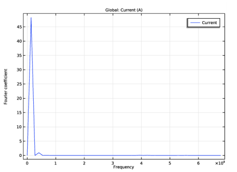
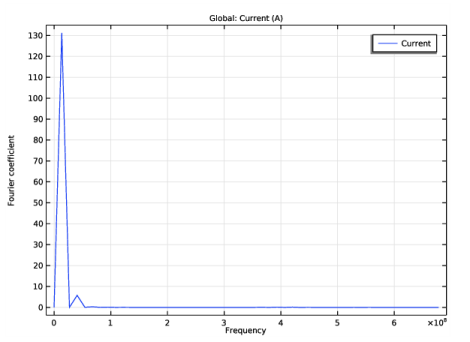
In the Settings window for 1D Plot Group, type Harmonic Content of the Current in the Label text field.
3
Locate the Data section. From the Dataset list, choose Time Periodic to Time Dependent/Solution 2 (sol2).
Global 1
1
Right-click Harmonic Content of the Current and choose Global.
2
In the Settings window for Global, click Replace Expression in the upper-right corner of the y-Axis Data section. From the menu, choose Component 1 (comp1)>Plasma, Time Periodic>Metal Contact 1>ptp.mct1.I - Current - A.
3
In the Harmonic Content of the Current toolbar, click  Plot.
4
Locate the x-Axis Data section. From the Parameter list, choose Discrete Fourier transform.
5
From the Show list, choose Frequency spectrum.
6
In the Harmonic Content of the Current toolbar, click  Plot.
7
Click the  Zoom Extents button in the Graphics toolbar.
For this low power value, the harmonic at 3 times the fundamental is only around 1.9% of the fundamental.
Next, use the FFT study so that the impedance of the discharge can be computed at the fundamental.
Add Study
1
In the Home toolbar, click  Add Study to open the Add Study window.
2
Go to the Add Study window.
3
Find the Studies subsection. In the Select Study tree, select Empty Study.
4
Click Add Study in the window toolbar.
5
In the Home toolbar, click  Add Study to close the Add Study window.
FFT Study to Compute Plasma Impedance
In the Settings window for Study, type FFT Study to Compute Plasma Impedance in the Label text field.
Time to Frequency FFT
1
In the Study toolbar, click  Study Steps and choose Frequency Domain>Time to Frequency FFT.
2
In the Settings window for Time to Frequency FFT, locate the Study Settings section.
3
In the End time text field, type 1/f0.
4
In the Maximum output frequency text field, type f0.
5
From the Input study list, choose Time Periodic to Time Dependent, Time Periodic to Time Dependent.
6
In the Study toolbar, click  Compute.
Results
Impedance (ptp, dset4)
After computing, a Global Evaluation feature is automatically generated, with the default expression corresponding to the plasma impedance. Evaluate this to the results table.
1
In the Settings window for Global Evaluation, click  Evaluate.
In order to recompute the plasma impedance for different operating conditions, it is necessary to run all three studies. To make this easier, a fourth study can be added, which uses the Study reference feature.
Add Study
1
In the Study toolbar, click  Add Study to open the Add Study window.
2
Go to the Add Study window.
3
Find the Studies subsection. In the Select Study tree, select Empty Study.
4
Click Add Study in the window toolbar.
5
In the Study toolbar, click  Add Study to close the Add Study window.
Run all Studies
In the Settings window for Study, type Run all Studies in the Label text field.
Now reference the first three studies. When computing this study, it will run the other three studies in order.
No Study
1
In the Study toolbar, click  Study Reference.
2
In the Settings window for Study Reference, locate the Study Reference section.
3
From the Study reference list, choose Time Periodic.
4
In the Study toolbar, click  Study Reference.
No Study
1
In the Settings window for Study Reference, locate the Study Reference section.
2
From the Study reference list, choose Time Periodic to Time Dependent.
3
In the Study toolbar, click  Study Reference.
No Study
1
In the Settings window for Study Reference, locate the Study Reference section.
2
From the Study reference list, choose FFT Study to Compute Plasma Impedance.
Now change the input power and recompute the studies.
Global Definitions
Parameters 1
1
In the Model Builder window, under Global Definitions click Parameters 1.
2
In the Settings window for Parameters, locate the Parameters section.
3
Run all Studies
In the Study toolbar, click  Compute.
Observe how the harmonic at 3 times the fundamental frequency has now increased to around 4.5% of the fundamental. This will cause significant problems with any potential matching network.
Results
Harmonic Content of the Current
Finally, reevaluate the plasma impedance at this new power value.
Impedance (ptp, dset4)
In the Model Builder window, under Results>Derived Values right-click Impedance (ptp, dset4) and choose Evaluate>Impedance - .