PDF

Global Model Coupled with the Two-Term Boltzmann Equation
Introduction
The electron energy distribution function (EEDF) plays an important role in the overall behavior of discharges. In this work, the formation period of an argon plasma with special attention for the EEDF is studied. The plasma is created within a 4 cm gap by a DC source voltage of 1 kV in series with a 100 kΩ resistance at 100 mTorr (compare with the Micro-cathode sustained discharge in Ar example from Ref. 1). A global model in the local field approximation is used to describe the temporal evolution of the plasma species. The rate coefficients for electron impact reactions and electron mobility are obtained from suitable integration of cross sections over the EEDF, and the EEDF is computed from the steady state Boltzmann equation in the two-term approximation (B2T) Ref. 2. The computed EEDF is influenced by how electrons gain energy from the electric field and lose it afterward in collisions with the background gas.
Coupling the B2T with a space dependent model is very computational expensive. Therefore, it is recommended to first explore the influence of the EEDF using a global (volume-averaged) model since it can run simulations in a fraction of the time of a space dependent model while retaining the tendencies of volume-averaged physical quantities.
Model Definition
The model used in this work considers that the spatial distribution of the different quantities in the plasma reactor can be treated as uniform or can be described using an analytic model. Without the spatial derivatives the numerical solution of the equation set becomes considerably simpler and the computation time is reduced. These advantages make a global model a good first approach to study a plasma reactor, especially when complex chemistries are involved or the influence of the EEDF is to be studied. In the following, we make use of the fast computational time to investigate the plasma evolution during the formation period through to steady state.
When using a plasma global model the species densities and the electron temperature are treated as volume-averaged quantities. Detailed information on the global model can be found in the section Theory for Global Models in the Plasma Module User’s Guide. For heavy species the following equation is solved for the mass fraction
where ρ is the mass density (SI unit: kg/m3), wk is the mass fraction, wf,k is the mass fraction in the feed, mf and mo are the mass-flow rates of the total feed and outlet, and Rk is the rate expression (SI unit: kg/(m3·s)). The fourth term on the right-hand side accounts for surface losses and creation, where Al is the surface area, hl is a dimensionless correction term, V is the reactor volume, Mk is the species molar mass (SI unit: kg/mol) and Rsurf,k,l is the surface rate expression (SI unit: mol/(m2·s)) at a surface l. The last term is introduced because the species mass balance equations are written in the nonconservative form and it used the mass-continuity equation to replace for the mass density time derivative. In the last term Mf,l is the inward mass flux of surface l (SI unit: kg/(m2·s)). The sum in the last two terms is over all surfaces where there are surface reactions.
To take possible variations of the system total mass or pressure into account, the mass-continuity equation can also be solved
.
The electron number density is obtained from electroneutrality
and if using the local energy approximation (LEA) the electron energy density nε (SI unit: V/ m3) is computed from
where Rε is the electron energy loss due to inelastic and elastic collisions, Pabs is the power absorbed by the electrons (SI unit: W), and e is the elementary charge. The last term on the right side accounts for the kinetic energy transported to the surface by electrons and ions. The summation is over all positive ions, εe is the mean kinetic energy lost per electron lost, εi is the mean kinetic energy lost per ion lost, and Na is Avogadro’s number. If using the local field approximation (LFA) the electron mean energy equation is not solved and the electron mean energy can be: (i) provided as a function of the electric field; or (ii) obtained by solving the Boltzmann equation in the two-term approximation.
The rate coefficients for electron impact reactions can be computed by appropriate averaging of cross sections over a EEDF. The EEDF can be either analytic or can be obtained by solving the steady state Boltzmann equation in the two-term approximation coupled with the equation system (The Boltzmann Equation, Two-Term Approximation Interface in the Plasma Module User’s Guide). When solving for the EEDF the coupling between the equations is as follows: (i) if the LEA is used the electron mean energy obtained from the electron mean energy equation is given as input to the Boltzmann solver; (ii) if the LFA is used the reduce electric field must be given as input to the Boltzmann solver and the electron mean energy comes from averaging over the computed EEDF.
In this work the LFA is used and the B2T is solved. The reduced electric field given as input to the B2T comes from the circuit equation
where Vp is the plasma potential, VDC is the applied voltage, and R is the circuit series resistance. The plasma current Ip is computed from
where e is the electron charge, A is the plasma cross section area, μN is the reduced electron mobility, E/N is the reduced electric field, and N is the gas density. Solving for E/N one obtains
where d is the gap distance. One can anticipate that an increase in the plasma density will reduce the electric field in the discharge gap.
plasma chemistry
The plasma chemistry suggested in Ref. 1 is used and presented in Table 1. The chemical mechanism consists of 5 species and 11 reactions.
The model also includes the surface reactions presented in Table 2.
The neutral excited species revert to ground state with sticking coefficient equal to one.
Results and Discussion
Figure 1 shows computed and analytic EEDFs for a mean electron energy of 5 eV. These results were obtained with the EEDF Initialization study that only solves for the Boltzmann equation in the two-term approximation without solving for the degrees of freedom from the global model. This approach allows to have a first insight of the EEDF and observe if an analytic EEDF is accurate enough for the modeling expectations. From Figure 1 it is possible to see that above 20 eV the computed EEDF drops much faster than the Maxwellian EEDF. As a consequence the Maxwellian EEDF overpredicts electron impact processes with high energy thresholds like ionization from the ground state. The Druyvesteyn EEDF is in much better agreement with the computed EEDF and it might be good enough for some models.
From Figure 2 to Figure 5, simulation results are presented for the global model coupled with the B2T. Figure 2 shows the temporal evolution of the plasma species and the reduced field in the plasma. In the first instants there is no plasma in the gap and the electric field maintains a constant value until the plasma creation begins. With the plasma creation the current in the gap (which is only plasma conduction current in this model) increases and the voltage decreases as presented in Figure 3. At steady state the plasma is sustained with only 30 V in the gap that corresponds to a field of 3.5 Td.
From Figure 4 it is possible to observe that the temporal evolution of the electron mean energy (obtained by averaging the computed EEDF) follows the same trend as the electric field. The electron mean energy decreases with the electric field and undershoots before reaching the steady state. The same behavior can be inferred from the temporal evolution of the EEDFs presented in Figure 5. Further analyses of the EEDF allows to gain a deeper understating of the plasma physics. In the beginning the electrons have a large population above 15 eV as it is necessary to facilitate the plasma breakdown. After the plasma formation, and due to the decrease of the electric field, the electron population cools down and the EEDF develops a tail with a steeper slope. As time progresses, and with the increase of the argon excited state density, the influence of the superelastic reactions in the EEDF becomes noticeable with the appearance of a bump at the high energy end.
Figure 1: Computed and analytic EEDFs for a mean electron energy of 5 eV.
Figure 2: Temporal evolution of the plasma species and the reduced electric field.
Figure 3: Temporal evolution of the plasma voltage and current.
Figure 4: Temporal evolution of the mean electron energy.
Figure 5: Computed EEDF at several instants of the simulation.
References
1. S. Pancheshnyi, B. Eismann, G.J.M. Hagelaar, and L.C. Pitchford, Computer code ZDPlasKin, http://www.zdplaskin.laplace.univ-tlse.fr (University of Toulouse, LAPLACE, CNRS-UPS-INP, Toulouse, France, 2008).
2. G.J.M. Hagelaar and L.C. Pitchford, “Solving the Boltzmann Equation to Obtain Electron Transport Coefficients and Rate Coefficients for Fluid Models”, Plasma Sources Science and Technology, vol. 14, pp. 722–733, 2005.
3. Phelps database, www.lxcat.net, retrieved 2017.
Application Library path: Plasma_Module/Global_Modeling/boltzmann_global_model_argon
Modeling Instructions
From the File menu, choose New.
New
In the New window, click  Model Wizard.
Model Wizard
1
In the Model Wizard window, Select the Plasma (plas) interface and the EEDF Initialization study.
2
click  2D Axisymmetric.
3
In the Select Physics tree, select Plasma>Plasma (plas).
4
Click Add.
5
Click  Study.
6
In the Select Study tree, select Preset Studies for Selected Physics Interfaces>EEDF Initialization.
7
Geometry 1
Create a geometry to define the plasma volume and contact surfaces.
Rectangle 1 (r1)
1
In the Geometry toolbar, click  Rectangle.
2
In the Settings window for Rectangle, locate the Size and Shape section.
3
In the Width text field, type rad.
4
In the Height text field, type gap.
Add some parameters to define the geometry, background gas temperature, and circuit components.
Global Definitions
Parameters 1
1
In the Model Builder window, under Global Definitions click Parameters 1.
2
In the Settings window for Parameters, locate the Parameters section.
3
Add some variables to define the diffusion length, the reduced electric field in the plasma, and the plasma current and voltage.
Definitions
Variables 1
1
In the Model Builder window, under Component 1 (comp1) right-click Definitions and choose Variables.
2
In the Settings window for Variables, locate the Variables section.
3
Choose to solve a global model in the local field approximation coupled with the electron Boltzmann equation in the two-term approximation.
Plasma (plas)
1
In the Model Builder window, under Component 1 (comp1) click Plasma (plas).
2
In the Settings window for Plasma, locate the Diffusion Model section.
3
From the Diffusion model list, choose Global.
4
Locate the Plasma Properties section. From the Mean electron energy list, choose Local field approximation.
5
Locate the Electron Energy Distribution Function Settings section. From the Electron energy distribution function list, choose Boltzmann equation, two-term approximation (linear).
6
In the εmax text field, type 50[V].
Import cross section data for argon.
Cross Section Import 1
1
In the Physics toolbar, click  Global and choose Cross Section Import.
2
In the Settings window for Cross Section Import, locate the Cross Section Import section.
3
Click  Browse.
4
5
Click  Import.
Add other reactions to complete the plasma chemistry.
Electron Impact Reaction 6
1
In the Physics toolbar, click  Domains and choose Electron Impact Reaction.
2
In the Settings window for Electron Impact Reaction, locate the Reaction Formula section.
3
In the Formula text field, type Ar++e+e=>Ar+e.
4
Locate the Collision Type section. From the Collision type list, choose Excitation.
5
In the Δε text field, type -15.8.
6
Locate the Reaction Parameters section. In the kf text field, type 8.75e-27[cm^6/s]*(plas.Te/1[V])^-4.5*N_A_const*N_A_const.
Electron Impact Reaction 7
1
In the Physics toolbar, click  Domains and choose Electron Impact Reaction.
2
In the Settings window for Electron Impact Reaction, locate the Reaction Formula section.
3
In the Formula text field, type Ar2++e=>Ars+Ar.
4
Locate the Collision Type section. From the Collision type list, choose Excitation.
5
In the Δε text field, type -3.
6
Locate the Reaction Parameters section. In the kf text field, type 8.5e-7[cm^3/s]*(plas.Te*11600[K/V]/300[K])^-0.67*N_A_const.
Reaction 1
1
In the Physics toolbar, click  Domains and choose Reaction.
2
In the Settings window for Reaction, locate the Reaction Formula section.
3
In the Formula text field, type Ar++Ar+Ar=>Ar2++Ar.
4
Locate the Reaction Parameters section. In the kf text field, type 2.25e-31[cm^6/s]*(Tg/300[K])^-0.4*N_A_const*N_A_const.
9: Ar++Ar+Ar=>Ar2++Ar
1
Right-click 8: Ar++Ar+Ar=>Ar2++Ar and choose Duplicate.
2
In the Settings window for Reaction, locate the Reaction Formula section.
3
In the Formula text field, type Ars+Ar+Ar=>Ar+Ar+Ar.
4
Locate the Reaction Parameters section. In the kf text field, type 1.4e-32[cm^6/s]*N_A_const*N_A_const.
10: Ars+Ar+Ar=>Ar+Ar+Ar
1
Right-click 9: Ars+Ar+Ar=>Ar+Ar+Ar and choose Duplicate.
2
In the Settings window for Reaction, locate the Reaction Formula section.
3
In the Formula text field, type Ars+Ars=>Ar2++e.
4
Locate the Reaction Parameters section. In the kf text field, type 6e-10[cm^3/s]*N_A_const.
11: Ars+Ars=>Ar2++e
1
Right-click 10: Ars+Ars=>Ar2++e and choose Duplicate.
2
In the Settings window for Reaction, locate the Reaction Formula section.
3
In the Formula text field, type Ar2++Ar=>Ar++Ar+Ar.
4
Locate the Reaction Parameters section. In the kf text field, type 6.06e-6[K*cm^3/s]/Tg*exp(-15130[K]/Tg)*N_A_const.
Species: Ar
1
In the Model Builder window, click Species: Ar.
2
In the Settings window for Species, locate the Species Formula section.
3
Select the From mass constraint check box.
4
Locate the General Parameters section. From the Preset species data list, choose Ar.
Species: Ars
1
In the Model Builder window, click Species: Ars.
2
In the Settings window for Species, locate the General Parameters section.
3
From the Preset species data list, choose Ar.
Species: Ar+
1
In the Model Builder window, click Species: Ar+.
2
In the Settings window for Species, locate the General Parameters section.
3
From the Preset species data list, choose Ar.
4
In the n0 text field, type 1e6[1/cm^3].
Species: Ar2+
1
In the Model Builder window, click Species: Ar2+.
2
In the Settings window for Species, locate the General Parameters section.
3
From the Preset species data list, choose Ar.
4
In the n0 text field, type 1E1[1/cm^3].
Define surface losses for ions and argon excited state.
Surface Reaction 1
1
In the Physics toolbar, click  Boundaries and choose Surface Reaction.
2
In the Settings window for Surface Reaction, locate the Boundary Selection section.
3
From the Selection list, choose All boundaries.
4
Locate the Reaction Formula section. In the Formula text field, type Ar+=>Ar.
5
From the Specify reaction using list, choose Sticking coefficient and diffusion.
6
Locate the Reaction Parameters section. In the Λeff text field, type Ldiff.
2: Ar+=>Ar
1
Right-click 1: Ar+=>Ar and choose Duplicate.
2
In the Settings window for Surface Reaction, locate the Reaction Formula section.
3
In the Formula text field, type Ar2+=>Ar+Ar.
3: Ar2+=>Ar+Ar
1
Right-click 2: Ar2+=>Ar+Ar and choose Duplicate.
2
In the Settings window for Surface Reaction, locate the Reaction Formula section.
3
In the Formula text field, type Ars=>Ar.
Set the gas temperature, the gas pressure, the reduced electric field for the EEDF, and the mean electron energy for the EEDF initialization.
Plasma Model 1
1
In the Model Builder window, click Plasma Model 1.
2
In the Settings window for Plasma Model, locate the Model Inputs section.
3
In the T text field, type Tg.
4
In the p0 text field, type P0.
5
Locate the EEDF Inputs section. In the E/N text field, type EN.
6
In the ε0 text field, type 5[V].
Compute the EEDF without solving for the other plasma degrees of freedom. This is a good first step to gain knowledge about the EEDF for the present conditions. The EEDF will also be used as an initial EEDF for the time dependent plasma model.
Study 1
In the Home toolbar, click  Compute.
Compare the computed EEDF with analytic EEDFs.
Results
EEDF initialization
1
In the Settings window for 1D Plot Group, type EEDF initialization in the Label text field.
2
Locate the Plot Settings section. In the x-axis label text field, type Energy (eV).
3
In the y-axis label text field, type EEDF (eV <sup>-3/2</sup>).
4
Click to expand the Title section. From the Title type list, choose None.
5
Locate the Axis section. Select the Manual axis limits check box.
6
In the x minimum text field, type 0.
7
In the x maximum text field, type 40.
8
In the y minimum text field, type 1e-12.
9
In the y maximum text field, type 0.5.
10
In the EEDF initialization toolbar, click  Plot.
Add a study to solve for the global model equations coupled with the Boltzmann equation.
Add Study
1
In the Home toolbar, click  Add Study to open the Add Study window.
2
Go to the Add Study window.
3
Find the Studies subsection. In the Select Study tree, select General Studies>Time Dependent.
4
Click Add Study in the window toolbar.
5
In the Home toolbar, click  Add Study to close the Add Study window.
Study 2
Step 1: Time Dependent
1
In the Settings window for Time Dependent, locate the Study Settings section.
2
Click  Range.
3
In the Range dialog box, choose Logarithmic from the Entry method list.
4
In the Start text field, type 1e-10.
5
In the Stop text field, type 0.001.
6
In the Steps per decade text field, type 20.
7
Click Replace.
8
In the Settings window for Time Dependent, click to expand the Values of Dependent Variables section.
9
Find the Initial values of variables solved for subsection. From the Settings list, choose User controlled.
10
From the Method list, choose Solution.
11
From the Study list, choose Study 1, EEDF Initialization.
12
In the Model Builder window, click Study 2.
13
In the Settings window for Study, locate the Study Settings section.
14
Clear the Generate default plots check box.
15
Clear the Generate convergence plots check box.
Solution 2 (sol2)
1
In the Study toolbar, click  Show Default Solver.
2
In the Model Builder window, expand the Solution 2 (sol2) node, then click Time-Dependent Solver 1.
3
In the Settings window for Time-Dependent Solver, click to expand the Time Stepping section.
4
From the Steps taken by solver list, choose Strict.
5
Click  Compute.
Results
Prepare a plot to show the temporal evolution of the species densities and the reduced electric field.
Species densities and E/N vs. time
1
In the Home toolbar, click  Add Plot Group and choose 1D Plot Group.
2
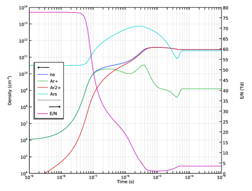
In the Settings window for 1D Plot Group, type Species densities and E/N vs. time in the Label text field.
3
Locate the Data section. From the Dataset list, choose Study 2/Solution 2 (sol2).
4
Locate the Title section. From the Title type list, choose None.
Global 1
1
Right-click Species densities and E/N vs. time and choose Global.
2
In the Settings window for Global, locate the y-Axis Data section.
3
Global 2
1
In the Model Builder window, right-click Species densities and E/N vs. time and choose Global.
2
In the Settings window for Global, locate the y-Axis Data section.
3
Species densities and E/N vs. time
1
In the Model Builder window, click Species densities and E/N vs. time.
2
In the Settings window for 1D Plot Group, locate the Plot Settings section.
3
Select the Two y-axes check box.
4
In the table, select the Plot on secondary y-axis check box for Global 2.
5
Select the y-axis label check box. In the associated text field, type Density (cm<sup>-3</sup>).
6
Locate the Axis section. Select the Manual axis limits check box.
7
In the x minimum text field, type 1e-9.
8
In the x maximum text field, type 1e-3.
9
In the y minimum text field, type 1e4.
10
In the y maximum text field, type 1e14.
11
In the Secondary y minimum text field, type 0.
12
In the Secondary y maximum text field, type 80.
13
Select the x-axis log scale check box.
14
Select the y-axis log scale check box.
15
Locate the Legend section. From the Position list, choose Middle left.
16
In the Species densities and E/N vs. time toolbar, click  Plot.
Plot the temporal evolution of the plasma voltage and current.
1D Plot Group 3
In the Home toolbar, click  Add Plot Group and choose 1D Plot Group.
Global 1
1
Right-click 1D Plot Group 3 and choose Global.
2
In the Settings window for Global, locate the y-Axis Data section.
3
Global 2
1
Right-click Global 1 and choose Duplicate.
2
In the Settings window for Global, locate the y-Axis Data section.
3
Plasma voltage and current vs. time
1
In the Model Builder window, under Results click 1D Plot Group 3.
2
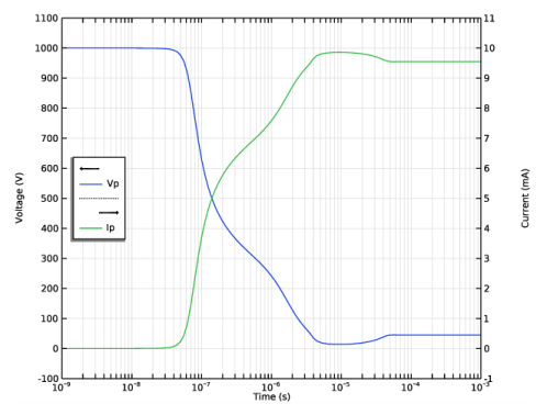
In the Settings window for 1D Plot Group, type Plasma voltage and current vs. time in the Label text field.
3
Locate the Data section. From the Dataset list, choose Study 2/Solution 2 (sol2).
4
Locate the Title section. From the Title type list, choose None.
5
Locate the Plot Settings section. Select the Two y-axes check box.
6
In the table, select the Plot on secondary y-axis check box for Global 2.
7
Select the y-axis label check box. In the associated text field, type Voltage (V).
8
Select the Secondary y-axis label check box. In the associated text field, type Current (mA).
9
Locate the Axis section. Select the Manual axis limits check box.
10
In the x minimum text field, type 1e-9.
11
In the x maximum text field, type 1e-3.
12
In the y minimum text field, type -100.
13
In the y maximum text field, type 1100.
14
In the Secondary y minimum text field, type -1.
15
In the Secondary y maximum text field, type 11.
16
Select the x-axis log scale check box.
17
Locate the Legend section. From the Position list, choose Middle left.
18
In the Plasma voltage and current vs. time toolbar, click  Plot.
Plot the temporal evolution of the electron mean energy.
Electron mean energy vs. time
1
In the Home toolbar, click  Add Plot Group and choose 1D Plot Group.
2
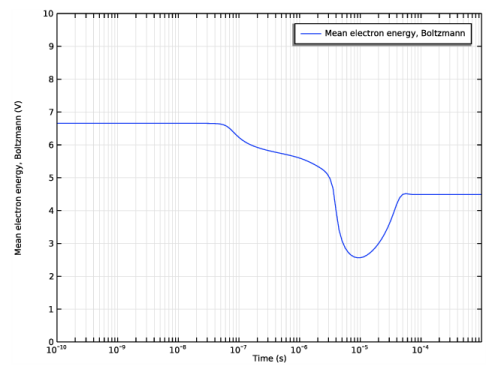
In the Settings window for 1D Plot Group, type Electron mean energy vs. time in the Label text field.
3
Locate the Data section. From the Dataset list, choose Study 2/Solution 2 (sol2).
4
Locate the Title section. From the Title type list, choose None.
5
Locate the Axis section. Select the Manual axis limits check box.
6
In the x minimum text field, type 1e-10.
7
In the x maximum text field, type 1e-3.
8
In the y minimum text field, type 0.
9
In the y maximum text field, type 10.
10
Select the x-axis log scale check box.
Global 1
1
Right-click Electron mean energy vs. time and choose Global.
2
In the Settings window for Global, locate the y-Axis Data section.
3
4
In the Electron mean energy vs. time toolbar, click  Plot.
Create a new dataset to plot the EEDF at several time instants.
Study 2/Solution 2 (4) (sol2)
1
In the Model Builder window, expand the Results>Datasets node.
2
Right-click Results>Datasets>Study 2/Solution 2 (sol2) and choose Duplicate.
3
In the Settings window for Solution, locate the Solution section.
4
From the Component list, choose Extra Dimension from Plasma (plas_eedf_xdim).
Plot the EEDF at several time instants.
EEDF vs. time
1
In the Home toolbar, click  Add Plot Group and choose 1D Plot Group.
2
In the Settings window for 1D Plot Group, type EEDF vs. time in the Label text field.
3
Locate the Data section. From the Dataset list, choose Study 2/Solution 2 (4) (sol2).
4
Locate the Title section. From the Title type list, choose None.
5
Locate the Data section. From the Time selection list, choose From list.
6
In the Times (s) list, choose 1E-10, 1E-7, 1E-6, 1E-5, and 0.001.
7
Locate the Plot Settings section.
8
Select the x-axis label check box. In the associated text field, type Energy (eV).
9
Select the y-axis label check box. In the associated text field, type EEDF (eV <sup>-3/2</sup>).
10
Locate the Axis section. Select the Manual axis limits check box.
11
In the x minimum text field, type 0.
12
In the x maximum text field, type 40.
13
In the y minimum text field, type 1e-12.
14
In the y maximum text field, type 0.5.
15
Select the y-axis log scale check box.
Line Graph 1
1
Right-click EEDF vs. time and choose Line Graph.
2
In the Settings window for Line Graph, locate the Selection section.
3
From the Selection list, choose All domains.
4
Locate the y-Axis Data section. In the Expression text field, type plas.fcap.
5
Locate the x-Axis Data section. From the Parameter list, choose Expression.
6
In the Expression text field, type plas.xeedf.
7
Click to expand the Legends section. Select the Show legends check box.
8
In the EEDF vs. time toolbar, click  Plot.