|
|
|

|
1
|
|
2
|
|
3
|
Click Add.
|
|
4
|
|
5
|
Click Add.
|
|
6
|
Click
|
|
7
|
|
8
|
Click
|
|
1
|
|
2
|
|
1
|
|
2
|
|
3
|
|
4
|
|
5
|
|
6
|
|
7
|
|
1
|
|
2
|
|
1
|
|
2
|
|
3
|
Click
|
|
4
|
Browse to the model’s Application Libraries folder and double-click the file mold_cooling_top.mphbin.
|
|
5
|
Click
|
|
6
|
Locate the Selections of Resulting Entities section. Find the Cumulative selection subsection. Click New.
|
|
7
|
|
8
|
Click OK.
|
|
9
|
|
10
|
|
11
|
Browse to the model’s Application Libraries folder and double-click the file mold_cooling_geom_sequence.mph.
|
|
12
|
|
13
|
|
14
|
|
1
|
|
2
|
|
3
|
|
4
|
|
5
|
Click OK.
|
|
1
|
|
2
|
|
3
|
|
4
|
|
1
|
|
2
|
|
3
|
|
1
|
|
1
|
|
2
|
In the tree, select Built-in>Aluminum.
|
|
3
|
|
4
|
|
5
|
|
6
|
|
1
|
In the Model Builder window, under Component 1 (comp1) right-click Materials and choose Blank Material.
|
|
2
|
|
3
|
|
4
|
|
1
|
|
2
|
|
3
|
|
1
|
In the Model Builder window, under Component 1 (comp1)>Nonisothermal Pipe Flow (nipfl) click Pipe Properties 1.
|
|
2
|
|
3
|
From the list, choose Circular.
|
|
4
|
|
5
|
|
6
|
|
1
|
|
2
|
|
3
|
|
4
|
|
1
|
|
2
|
|
3
|
|
1
|
|
3
|
|
4
|
|
5
|
|
1
|
|
1
|
|
2
|
|
3
|
|
1
|
In the Model Builder window, under Component 1 (comp1)>Heat Transfer in Solids (ht) click Initial Values 1.
|
|
2
|
|
3
|
|
1
|
|
2
|
|
3
|
|
4
|
|
5
|
|
1
|
|
2
|
|
3
|
|
1
|
|
2
|
|
3
|
|
1
|
|
1
|
|
2
|
|
3
|
Click the Custom button.
|
|
4
|
|
5
|
|
6
|
|
1
|
|
2
|
|
3
|
|
1
|
|
2
|
|
3
|
|
4
|
Click Replace Expression in the upper-right corner of the Expression section. From the menu, choose Component 1 (comp1)>Heat Transfer in Solids>Temperature>T2 - Temperature - K.
|
|
5
|
Locate the Expression section.
|
|
6
|
|
1
|
|
2
|
|
3
|
|
1
|
|
2
|
|
3
|
|
4
|
Click
|
|
5
|
Click
|
|
7
|
|
8
|
Locate the Study Settings section. Find the Memory settings for jobs subsection. From the Keep solutions list, choose Only last.
|
|
1
|
|
2
|
|
3
|
Click
|
|
1
|
|
2
|
|
3
|
In the Model Builder window, expand the Study 1>Solver Configurations>Solution 1 (sol1)>Time-Dependent Solver 1 node, then click Fully Coupled 1.
|
|
4
|
|
5
|
|
6
|
|
7
|
|
1
|
|
2
|
|
3
|
|
1
|
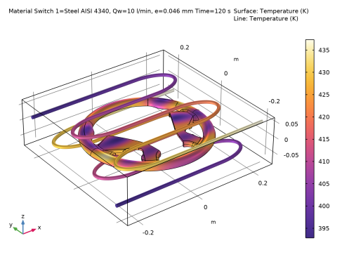
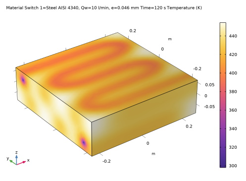
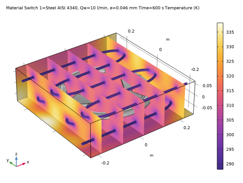
In the Settings window for 3D Plot Group, type Wheel and Cooling Channels Temperature in the Label text field.
|
|
2
|
|
3
|
|
1
|
|
2
|
|
3
|
|
4
|
|
5
|
|
6
|
|
7
|
|
1
|
|
2
|
|
3
|
|
4
|
|
5
|
|
6
|
Click to expand the Inherit Style section. Locate the Coloring and Style section. From the Scale list, choose Logarithmic.
|
|
7
|
|
8
|
|
9
|
|
10
|
|
11
|
|
12
|
|
1
|
In the Model Builder window, right-click Results and choose Add Predefined Plot>Study 1/Parametric Solutions 1 (sol2)>Heat Transfer in Solids>Temperature (ht).
|
|
2
|
|
3
|
|
4
|
|
5
|
|
6
|
|
7
|
|
1
|
Right-click Results and choose Add Predefined Plot>Study 1/Parametric Solutions 1 (sol2)>Pipe Wall Heat Transfer 1>Temperature (pwhtc1).
|
|
2
|
|
3
|
|
4
|
|
1
|
|
2
|
|
3
|
|
4
|
|
5
|
|
1
|
|
2
|
|
3
|
|
4
|
|
1
|
|
2
|
|
3
|
|
4
|
|
1
|
|
3
|
|
1
|
|
2
|
|
3
|
|
4
|
Click
|
|
1
|
|
2
|
|
3
|
Find the Filled table structure subsection. From the Parameter value list, choose 2: matsw.comp1.sw1=1, Qw=10.
|
|
1
|
|
2
|
|
3
|
Find the Filled table structure subsection. From the Parameter value list, choose 3: matsw.comp1.sw1=2, Qw=20.
|
|
1
|
|
2
|
|
3
|
Find the Filled table structure subsection. From the Parameter value list, choose 4: matsw.comp1.sw1=2, Qw=10.
|
|
1
|
In the Model Builder window, expand the Results>Probe Plot Group 1 node, then click Probe Table Graph 1.
|
|
2
|
|
3
|
|
4
|
|
5
|
|
7
|
|
1
|
|
2
|
|
3
|
|
4
|
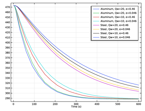
Locate the Legends section. In the table, enter the following settings:
|
|
1
|
|
2
|
|
3
|
|
4
|
Locate the Legends section. In the table, enter the following settings:
|
|
1
|
|
2
|
|
3
|
|
4
|
Locate the Legends section. In the table, enter the following settings:
|
|
1
|
|
2
|