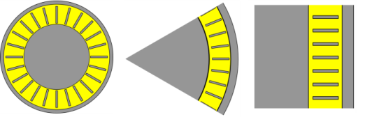
PDF

Quasi-2D Turbomolecular Pump
Introduction
Turbomolecular pumps are widely used in vacuum system design. A turbomolecular pump is a bladed molecular turbine that compresses gases by momentum transfer from the rapidly rotating blades of the rotor to the gas molecules. In the free molecular flow range (typically < 10-1 Pa), the particles collide primarily with the rotor resulting in an efficient pumping process. The following assumptions are made:
The Mathematical Particle Tracing interface can be used to evaluate the performance of a simple turbomolecular pump in the free molecular flow regime. While the Molecular Flow Module provides access to efficient and deterministic calculation of gas density in the free molecular flow regime, it uses the angular coefficient method which is only applicable for molecules or atoms that are moving much faster than any object in the model geometry. For turbopumps, where the blades move over similar time scales as the atoms or molecules themselves, this requirement is not satisfied, so a Monte Carlo approach is used instead.
This example is formulated as a quasi-2D model. That is, each turbine blade is very large compared to the root-to-tip distance, so it is a fair approximation to treat part of the turbine as an inertial frame of reference in which the blades are parallel, neglecting the effects of blade rotation.
The example Turbomolecular Pump shows how to set up a complete 3D model of a pump stage, complete with the centrifugal and Coriolis forces that arise when tracing particles in a noninertial frame of reference.
Model Definition
Modern turbomolecular pumps contain a large number of blades organized into stages, with adjacent stages sometimes rotating in opposite directions, or as rotor-stator pairs.
For a series of compression stages at zero flow, the overall compression ratio is approximately the product of the compression ratios for each stage (Ref. 1), so the overall performance of the pump can be investigated using a numerical model of a single stage. Thus, in this example only a single row of blades is considered. Furthermore, because of sector symmetry only the space between a single pair of adjacent blades is considered.
Blade Geometry
Typical cross sections of a pump stage are shown for three different radii of curvature in Figure 1. The empty space where molecules are free to propagate is in yellow, and solid domains are in gray. The blades (shown as thin gray rectangles) appear straight in such a cross section taken from above or below the stage, but a side view would reveal them to be inclined.
In the leftmost image, the blade radius (the distance from the center of rotation to the blade root, or the beginning of the empty space) is larger than the blade spacing, but not immensely so. In a co-rotating coordinate system, the centrifugal and Coriolis forces for this stage would be quite significant.
In the middle image, a sector from a pump stage with a much larger radius is shown. The curvature of this section is still evident, but not as greatly so as in the left image.
In the rightmost image, the radius of the pump stage has been taken to be arbitrarily large. Then the ring of blades takes on the appearance of an infinite straight row of blades having only translational velocity.
Figure 1: Cross sections of a single stage pump for varying radii of curvature.
This example uses the approximation of a pump stage with a large radius as an infinite row of blades, so that the co-moving frame of reference attached to the blades can be treated as inertial. The main advantage of this approximation is that molecules travel in straight lines in the co-moving frame, allowing the Time-Dependent Solver to accurately resolve the molecule trajectories even when taking very large time steps.
The Free Molecular Flow Regime
As illustrated in Figure 2, a turbomolecular pump causes a pressure difference between the domains on either side, depending on the angle, spacing, and speed of the moving blades. In the numerical model used here, the length scales are assumed to follow the relation
where
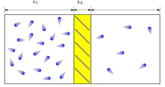
L1 is a characteristic length scale of either domain adjacent to the pump,
L2 is a characteristic length scale within a stage of the pump, and
λ (SI unit: m) is the molecular mean free path.
Because the mean free path is much smaller than length scales outside the pump, it is reasonable to assume that the gas in each adjacent domain is Maxwellian. This can be used to prescribe appropriate initial conditions for entering molecules. Because the mean free path is much larger than the length scales in each pump stage, it is also reasonable to neglect intermolecular collisions within the stage.
If the gas density were higher, so that the pump stage operates in the transitional flow regime instead of the free molecular flow regime, then it would still be possible to compute the transmission probability, but this would require intermolecular collisions to be included in the modeling domain, most likely with a Monte Carlo approach.
Figure 2: A single stage of a turbomolecular pump, consisting of a row of inclined blades, creates a pressure difference between the two adjacent domains. Not drawn to scale.
Model Parameters
The blade geometry is characterized by the blade length B (SI unit: m), blade spacing S (SI unit: m), and blade angle α (SI unit: rad), as shown in Figure 3.
Figure 3: Geometry parameters for the single-stage turbomolecular pump (side view).
In order to compute these transmission probabilities, the model uses an Inlet feature defined on at one end of the space between two blades, and uses the Outlet and Particle Counter to gather information about particles that reach the opposite side. The overall transmission probability is the ratio of the number of molecules that reach the Outlet boundary to the total number of released molecules.
Hydrogen gas molecules (H2) are released using an Inlet feature with the built-in Thermal velocity distribution. Similarly, the blade surfaces use a dedicated boundary condition called Thermal Re-Emission that randomly changes the particle’s speed and direction. Both the release feature and boundary condition launch molecules into the modeling domain with a distribution of directions following Knudsen’s cosine law, and with speeds sampled from the distribution
It is convenient to express the model parameters as dimensionless quantities. The blade length and spacing are related by a dimensionless blade aspect ratio S0,
The blade speed is expressed in terms of the dimensionless speed factor C,
where vp (SI unit: m/s) is the most probable speed of particles in the Maxwellian distribution,
where
kB = 1.380649 × 1023 J/K is the Boltzmann constant,
M = 2 g/mol is the approximate molar mass of the hydrogen gas, and
NA = 6.02214076 × 1023 1/mol is the Avogadro constant.
For hydrogen gas, this gives a most probable speed of approximately vp = 1579.3 m/s.
Results and Discussion
The model includes three studies, each with a separate Parametric Sweep. The parameter values used in these three studies are shown in Table 1 below. These values are almost identical to the values used to produce Figures 5-7 in Ref. 2.
The transmission probability as a function of speed factor C is shown in Figure 4. Compare this to Figure 5 in Ref. 2. Two curves are shown, the transmission probability M12 and the direct transmission probability m12 (both dimensionless). Particles only contribute to the direct transmission probability if they pass through the blades without ever hitting them, hence it reaches a maximum around C = 1 when the blade speed and most probable molecule speed are equal.
The transmission probability as a function of blade angle a is shown in Figure 5. Compare this to Figure 6 in Ref. 2. In both figures, the direct transmission probability reaches a maximum at about α = 35°, whereas the overall transmission probability reaches a maximum at the steeper angle α = 45°.
The transmission probability as a function of blade aspect ratio is shown in Figure 6. Compare this to Figure 7 in Ref. 2. (Note that, in the reference, the blade angle has been changed to 30°, whereas in this example it is maintained at 35° to be consistent with the first study.) When the blades are placed closer together, the overall transmission probability is decreased, and the direct transmission probability even more so, because it becomes very likely for a molecule to pass through without hitting the closely spaced blades.
Figure 4: Transmission probability of a single-stage pump as a function of the dimensionless velocity factor C.
Figure 5: Transmission probability of a single-stage pump as a function of the blade angle α.
Figure 6: Transmission probability of a single-stage pump as a function of the blade aspect ratio S0.
References
1. J.F. O’Hanlon, A user’s guide to vacuum technology, John Wiley & Sons, 2005.
2. S. Katsimichas, A.J.H. Goddard, R. Lewington, and C.R.E. De Oliveira, “General geometry calculations of one-stage molecular flow transmission probabilities for turbomolecular pumps,” Journal of Vacuum Science & Technology A: Vacuum, Surfaces, and Films, vol. 13, no. 6, pp. 2954–2961, 1995.
3. Li, Yanwu, Xuekang Chen, Yanhui Jia, Mingzheng Liu, and Zhong Wang. “Numerical investigation of three turbomolecular pump models in the free molecular flow range.” Vacuum, vol. 101, pp. 337-344, 2014.
Application Library path: Particle_Tracing_Module/Vacuum_Systems/turbomolecular_pump_quasi_2d
Modeling Instructions
From the File menu, choose New.
New
In the New window, click  Model Wizard.
Model Wizard
1
In the Model Wizard window, click  3D.
2
In the Select Physics tree, select Mathematics>Mathematical Particle Tracing (pt).
3
Click Add.
4
Click  Study.
5
In the Select Study tree, select General Studies>Time Dependent.
6
Global Definitions
Parameters 1
1
In the Model Builder window, under Global Definitions click Parameters 1.
2
In the Settings window for Parameters, locate the Parameters section.
3
Click  Load from File.
4
Definitions
Define some variables that will be used later for results analysis.
Variables 1
1
In the Model Builder window, under Component 1 (comp1) right-click Definitions and choose Variables.
2
In the Settings window for Variables, locate the Variables section.
3
The transmission probability is the fraction of molecules that reach the other side of the turbomolecular pump stage. The direct transmission probability is the fraction of molecules that cross the stage without hitting any of the blades.
At this point, the variable definitions will give a warning indicating an unknown variable. Any unknown variables will be defined later while setting up the physics.
Geometry 1
1
In the Model Builder window, under Component 1 (comp1) click Geometry 1.
2
In the Settings window for Geometry, locate the Units section.
3
From the Length unit list, choose cm.
The model geometry is an extrusion of a 2D polygon.
Work Plane 1 (wp1)
1
In the Geometry toolbar, click  Work Plane.
The default work plane orientation is used. With this orientation, the direction across the pump stage is the x direction, consecutive blades in the stage are offset in the y direction, and the geometry is considered uniform in the z direction.
Work Plane 1 (wp1)>Plane Geometry
In the Model Builder window, click Plane Geometry.
Work Plane 1 (wp1)>Polygon 1 (pol1)
1
In the Work Plane toolbar, click  Polygon.
2
In the Settings window for Polygon, locate the Coordinates section.
3
4
In the Work Plane toolbar, click  Build All.
Extrude 1 (ext1)
1
In the Model Builder window, under Component 1 (comp1)>Geometry 1 right-click Work Plane 1 (wp1) and choose Extrude.
2
In the Settings window for Extrude, click  Build All Objects.
Mathematical Particle Tracing (pt)
Particle Properties 1
1
In the Model Builder window, under Component 1 (comp1)>Mathematical Particle Tracing (pt) click Particle Properties 1.
2
In the Settings window for Particle Properties, locate the Particle Mass section.
3
In the mp text field, type mp_H2.
Before setting up the particle releases and boundary conditions, define an additional dependent variable that will be used to identify particles that pass through the stage without ever hitting a blade.
Auxiliary Dependent Variable 1
1
In the Physics toolbar, click  Global and choose Auxiliary Dependent Variable.
2
In the Settings window for Auxiliary Dependent Variable, locate the Auxiliary Dependent Variable section.
3
In the Field variable name text field, type noCollision.
This auxiliary variable noCollision will be initialized to 1 for released particles and reinitialized to 0 if they hit the blades. It was used previously in the definition of m12.
Release molecules from one side of the pump stage. The gas in the adjoining domain is assumed to follow a Maxwellian distribution, so that the speeds of incoming molecules are randomly sampled based on the surrounding temperature.
Inlet 1
1
In the Physics toolbar, click  Boundaries and choose Inlet.
Define an Inlet boundary condition to release the molecules at x = 0.
2
3
In the Settings window for Inlet, locate the Initial Position section.
4
From the Initial position list, choose Random.
5
In the N text field, type Np.
6
Locate the Initial Velocity section. From the Initial velocity list, choose Thermal.
7
In the T text field, type T0.
8
Locate the Initial Value of Auxiliary Dependent Variables section. In the noCollision0 text field, type 1.
The space between two adjacent blades is an inertial frame moving at constant velocity relative to the laboratory frame. Subtract the relative velocity between the two frames from the initial particle velocity.
9
Click to expand the Advanced Settings section. Select the Subtract moving frame velocity from initial particle velocity check box.
10
From the Background velocity list, choose User defined.
11
Specify the vb vector as
Wall 1 (Symmetry Boundaries)
1
In the Model Builder window, click Wall 1.
2
In the Settings window for Wall, type Wall 1 (Symmetry Boundaries) in the Label text field.
3
Locate the Wall Condition section. From the Wall condition list, choose Bounce.
The surfaces parallel to the xy-plane are treated as symmetry boundaries because the blade extends arbitrarily far in the z direction.
Use the Thermal Re-Emission boundary condition to resample the particle velocity from a distribution based on temperature at the blades.
Thermal Re-Emission 1 (Blade Surfaces)
1
In the Physics toolbar, click  Boundaries and choose Thermal Re-Emission.
2
3
In the Settings window for Thermal Re-Emission, locate the Wall Properties section.
4
In the T text field, type T0.
5
In the Label text field, type Thermal Re-Emission 1 (Blade Surfaces).
6
Click to expand the New Value of Auxiliary Dependent Variables section. Select the Assign new value to auxiliary variable : noCollision check box. Use the default value, 0.
Outlet 1
1
In the Physics toolbar, click  Boundaries and choose Outlet. The Outlet will stop particles when they either cross the pump stage completely or get deflected back to the Inlet boundary.
2
Particle Counter 1
1
In the Physics toolbar, click  Boundaries and choose Particle Counter.
2
This Particle Counter does not affect particle trajectories in any way, but it defines some additional variables that are useful for postprocessing. In particular, this step resolves any unknown variable issues in the Variables 1 node.
Mesh 1
1
In the Model Builder window, under Component 1 (comp1) click Mesh 1.
2
In the Settings window for Mesh, locate the Physics-Controlled Mesh section.
3
From the Element size list, choose Extremely coarse. The mesh quality is not important because all of the surfaces in the model are flat, and because no field variables are solved for in the domain. Hence a very coarse mesh can be used.
4
Click  Build All.
Sweep Over Speeds
In the remaining steps, set up three separate parametric sweeps to analyze the effects of the velocity, angle, and spacing of blades on the transmission probability of the single-stage pump. Begin with a Parametric Sweep over the dimensionless blade velocity C.
1
In the Model Builder window, click Study 1.
2
In the Settings window for Study, type Sweep Over Speeds in the Label text field.
3
Locate the Study Settings section. Clear the Generate default plots check box.
Parametric Sweep
1
In the Study toolbar, click  Parametric Sweep.
2
In the Settings window for Parametric Sweep, locate the Study Settings section.
3
4
Step 1: Time Dependent
1
In the Model Builder window, click Step 1: Time Dependent.
2
In the Settings window for Time Dependent, locate the Study Settings section.
3
From the Time unit list, choose ms.
4
In the Output times text field, type 0 0.2.
5
In the Study toolbar, click  Compute.
Results
Transmission Probability: Sweep Over Speeds
1
In the Home toolbar, click  Add Plot Group and choose 1D Plot Group.
2
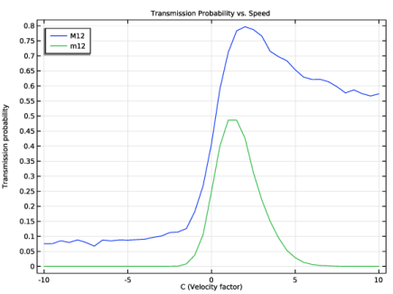
In the Settings window for 1D Plot Group, type Transmission Probability: Sweep Over Speeds in the Label text field.
3
Locate the Data section. From the Dataset list, choose Sweep Over Speeds/Parametric Solutions 1 (sol2).
4
From the Time selection list, choose Last.
5
Click to expand the Title section. From the Title type list, choose Manual.
6
In the Title text area, type Transmission Probability vs. Speed.
7
Locate the Plot Settings section.
8
Select the y-axis label check box. In the associated text field, type Transmission probability.
9
Locate the Legend section. From the Position list, choose Upper left.
Global 1
1
Right-click Transmission Probability: Sweep Over Speeds and choose Global.
2
In the Settings window for Global, locate the y-Axis Data section.
3
4
Locate the x-Axis Data section. From the Axis source data list, choose Outer solutions.
5
Click to expand the Legends section. From the Legends list, choose Manual.
6
7
In the Transmission Probability: Sweep Over Speeds toolbar, click  Plot. Compare the resulting image to Figure 4.
Root
Repeat the previous steps with a new Parametric Sweep over the blade angle alpha.
Add Study
1
In the Home toolbar, click  Add Study to open the Add Study window.
2
Go to the Add Study window.
3
Find the Studies subsection. In the Select Study tree, select General Studies>Time Dependent.
4
Click Add Study in the window toolbar.
5
In the Home toolbar, click  Add Study to close the Add Study window.
Sweep Over Angles
1
In the Model Builder window, click Study 2.
2
In the Settings window for Study, type Sweep Over Angles in the Label text field.
3
Locate the Study Settings section. Clear the Generate default plots check box.
Parametric Sweep
1
In the Study toolbar, click  Parametric Sweep.
2
In the Settings window for Parametric Sweep, locate the Study Settings section.
3
4
Step 1: Time Dependent
1
In the Model Builder window, click Step 1: Time Dependent.
2
In the Settings window for Time Dependent, locate the Study Settings section.
3
From the Time unit list, choose ms.
4
In the Output times text field, type 0 0.2.
5
In the Study toolbar, click  Compute.
Results
Transmission Probability: Sweep Over Angles
1
In the Model Builder window, right-click Transmission Probability: Sweep Over Speeds and choose Duplicate.
2
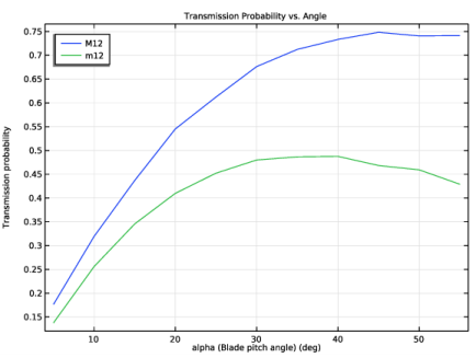
In the Settings window for 1D Plot Group, type Transmission Probability: Sweep Over Angles in the Label text field.
3
Locate the Data section. From the Dataset list, choose Sweep Over Angles/Parametric Solutions 2 (sol45).
4
Locate the Title section. In the Title text area, type Transmission Probability vs. Angle.
5
In the Transmission Probability: Sweep Over Angles toolbar, click  Plot. Compare the resulting image to Figure 5.
Root
Conclude with a third Parametric Sweep over the dimensionless aspect ratio S0, which is the ratio of the spacing between adjacent blades to the length of each blade.
Add Study
1
In the Home toolbar, click  Add Study to open the Add Study window.
2
Go to the Add Study window.
3
Find the Studies subsection. In the Select Study tree, select General Studies>Time Dependent.
4
Click Add Study in the window toolbar.
5
In the Home toolbar, click  Add Study to close the Add Study window.
Sweep Over Aspect Ratios
1
In the Model Builder window, click Study 3.
2
In the Settings window for Study, type Sweep Over Aspect Ratios in the Label text field.
3
Locate the Study Settings section. Clear the Generate default plots check box.
Parametric Sweep
1
In the Study toolbar, click  Parametric Sweep.
2
In the Settings window for Parametric Sweep, locate the Study Settings section.
3
4
Step 1: Time Dependent
1
In the Model Builder window, click Step 1: Time Dependent.
2
In the Settings window for Time Dependent, locate the Study Settings section.
3
From the Time unit list, choose ms.
4
In the Output times text field, type 0 0.2.
5
In the Study toolbar, click  Compute.
Results
Transmission Probability: Sweep Over Aspect Ratios
1
In the Model Builder window, right-click Transmission Probability: Sweep Over Speeds and choose Duplicate.
2
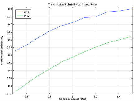
In the Settings window for 1D Plot Group, type Transmission Probability: Sweep Over Aspect Ratios in the Label text field.
3
Locate the Data section. From the Dataset list, choose Sweep Over Aspect Ratios/Parametric Solutions 3 (sol58).
4
Locate the Title section. In the Title text area, type Transmission Probability vs. Aspect Ratio.
5
In the Transmission Probability: Sweep Over Aspect Ratios toolbar, click  Plot. Compare the resulting image to Figure 6.