PDF

Three-Body Problem
Introduction
The motion of two objects under the influence of each others’ gravitational attraction is a classic problem with well-known analytic solutions, the Kepler orbits. In general, the motion of three or more objects under mutual gravitational attraction does not have a closed-form analytic solution.
The three-body problem is an example of a chaotic system; for most initial positions and velocities of the three objects, their motion will never exactly repeat itself, and a very slight change to the initial conditions can result in a drastic change in their behavior at some later time. However, there are specific arrangements of the three objects that will repeat themselves, known as periodic solutions to the three-body problem.
In this example, we solve the three-body problem numerically for three stars of equal mass using the Mathematical Particle Tracing interface. The gravitational force between the stars is implemented using the Particle-Particle Interaction node with user-defined expressions. The stars are arranged in two different sets of initial conditions corresponding to known periodic solutions to the three-body problem: the figure-eight configuration and the Lagrange configuration.
Model Definition
In this example, the positions and velocities of three points, representing stars, are solved for over time. The motion of each star follows the solution to two coupled first order differential equations for the position qi (SI unit: m) and the velocity vi (SI unit: m/s),
where i is a unique index for each star, mi (SI unit: kg) is the mass, and Fi (SI unit: N) is the total force exerted on the star. In this example, the only forces on each star are the attractive gravitational forces exerted on it by the other two stars in the system,
where in this example N = 3 and the index i = j is excluded from the sum. N-body configurations are sometimes reported in dimensionless coordinates by assuming each body has unit mass and that the gravitational constant is unity, but in this example the actual value of Newton’s gravitational constant is used, G = 6.67408 × 10-11 m3/(kg s2).
Existence of Analytic Solutions
If N = 2 (the two-body problem), then the equations of motion of the two stars can be solved analytically to obtain Kepler orbits. The trajectories of the two stars are conic sections (usually an ellipse or hyperbola) with a focus at the center of mass of the system.
If N = 3 (the three-body problem), then in general the equations of motion of the three stars cannot be solved analytically, and numerical methods are required. Three-body systems often exhibit chaotic motion: for most initial conditions, the motion of the three stars will never exactly repeat itself, and even a slight change in the initial position or velocity of one star can cause the trajectories to look completely different at some later time.
However, there do exist some particular sets of initial positions and velocities, for which the motion of three bodies would repeat itself. These are called periodic solutions to the three-body problem. Periodic solutions to the three-body problem may further be categorized as either stable or unstable. A stable periodic solution may continue to repeat itself for a large number of orbits even if the initial positions and velocities are not perfect (although there is some limit to how much they can be perturbed). An unstable periodic solution will be distorted beyond recognition in just a few orbital periods if the initial conditions are even slightly perturbed.
The Figure-Eight
In the figure-eight configuration, three stars of equal mass chase each other along a single self-intersecting path in the shape of the number 8 or an infinity symbol. The figure-eight configuration is considered stable because the stars will still follow approximately the same path for a large number of orbital periods even if the initial positions are slightly incorrect. However, there is a limit to this region of stability, so a very large error in the initial positions can still result in the stars following a chaotic pattern.
The initial positions and velocities that give rise to a stable figure-eight are given in Ref. 1:
with xi and yi the initial coordinates; ui and vi are the initial velocity components; and T is the orbital period. Note that these initial values are given for a dimensionless system in which G = 1, m = 1, and the initial distance from the center star to either of the other stars is exactly 1. To get the initial velocity components and period in a real system where the gravitational constant is G = 6.67408 × 10-11 m3/(kg s2), the stars each have the mass of the sun (about m = 1.989 × 1030 kg), and the initial distance between stars is about 30 astronomical units (1 AU = 149,597,870,700 m), we apply the following scale factors:
The Lagrange Configuration
In the Lagrange configuration, three stars of equal mass are positioned at the vertices of an equilateral triangle. The initial velocities are prescribed so that this triangle of stars rotates around its center of mass. The vertices of this triangle may stay at a fixed size (in which case the stars follow circular orbits) or may repeatedly shrink and expand (in which case the stars follow three identical elliptical orbits that intersect each other) depending on the initial speed. This setup is illustrated in Figure 1.
Figure 1: Initial star positions and velocities in the Lagrange configuration.
The Lagrange configuration is inherently unstable: if two of the stars are even slightly closer to each other, than they are to the third star, then within the span of a few orbital periods the star positions will usually not resemble the Lagrange configuration at all.
In this example, the initial velocity is defined so that the stars in the Lagrange configuration follow circular paths rather than elliptical paths. First the velocity is determined so that the inward gravitational force (toward the center of mass) equals the centrifugal force on the stars in their rotating frame of reference.
If the distance from any star to the center of mass is R, then the distance between stars, that is, the lengths of the sides of the equilateral triangle, are all . Now suppose that all three stars have equal mass, that is m1 = m2 = m3 = m. The three stars are assumed to orbit in the xy-plane with the first star lying along the positive x-axis. The total gravitational force on the first star is then
where i and j are unit vectors in the x and y directions. Further simplification yields
In order for the three stars to orbit the center of mass in a circle, the inward gravitational force must counterbalance the fictitious centrifugal force,
Solving for the speed V then yields
The period is the time required to complete one circular orbit,
If a smaller initial velocity is used, the orbits will be three ellipses that intersect each other, each with one focus at the center of mass of the triangular arrangement of stars.
Results and Discussion
In the first study, the stars are released in the figure-eight configuration. The result after ten periods is shown in Figure 2. The stars continue to trace the same path with no visible deviation from this path. A possible extension to this model would be to slightly perturb the mass, initial positions, or initial velocities, and observe whether the stars continue to follow the figure-eight or begin showing chaotic motion.
Figure 2: Trajectories of three stars of equal mass in the periodic “figure-eight” configuration.
An important consideration in any orbital simulation is the time stepping algorithm used and the time step size taken by the solver. In this example, the Newtonian, first order formulation was used, which uses the Dormand-Prince 5 Runge–Kutta time-stepping algorithm by default. A very tight relative tolerance of 10-10 was also specified in the study step’s settings to help improve the accuracy of the solution.
One viable figure-of-merit for checking the accuracy of the solution is the total energy of the system. To report total energy, it is necessary to include both kinetic energy and gravitational potential energy,
It is important to avoid double-counting the gravitational potential energy between any pair of particles when evaluating the total potential energy of the system.
A plot of the change in total energy versus time is shown in Figure 3. The relative change in total energy at the last time step is on the order of 10-9, and can be improved by further reducing the Relative tolerance in the settings for the Time Dependent study step.
Figure 3: Relative change in total energy of the “figure-eight” configuration of stars.
The trajectory plot in Figure 4 shows the Lagrange configuration after ten periods. In the model, it is also possible to plot the trajectories at an earlier time or to play an animation, showing that the three stars actually do follow a circular path for several periods. At about seven orbital periods, the minuscule numerical errors (recall that the tolerance is 10-10) begin to cause two of the stars to be visibly closer to each other than they are to the third star. The two closer stars will exert a stronger gravitational force on each other, bringing them even closer to each other in a positive feedback loop.
Eventually, the circular configuration collapses, with two of the stars repeatedly passing close to each other and then being launched away at high speed. Depending on the exact solver settings used, the trajectory plot might not look exactly the same as it does in Figure 4, but the basic principle remains the same: due to the inherent instability of the Lagrange configuration, small numerical errors accumulate over time and eventually cause the orderly equilateral triangle of stars to violently shake itself apart.
Figure 4: Trajectories of three stars of equal mass in the unstable Lagrange configuration.
Notes About the COMSOL Implementation
There is specific syntax which must be used to specify user-defined interaction forces with the Particle-Particle Interaction node. Recall that the expression for the gravitational force is
To implement this expression in the Particle-Particle Interaction, enter the components
gravity*pt.mp*dest(pt.mp)*(qx-dest(qx))/pt.r^3
gravity*pt.mp*dest(pt.mp)*(qy-dest(qy))/pt.r^3
Note that this expression uses a special operator called dest(), which stands for “destination”. When computing the total force on a particle, you may think of dest(qx) as “this particle’s x-coordinate” and qx as “any other particle’s x-coordinate”. The Particle-Particle Interaction node then computes the sum of the force contributions from all other particles. To help make expressions like this one more concise, the variable pt.r in the denominator is automatically defined as
pt.r = sqrt(1.0E-50+pt.dqx^2+pt.dqy^2+pt.dqz^2)
pt.dqx = qx-dest(qx)
pt.dqy = qy-dest(qy)
pt.dqz = qz-dest(qz)
with the last line simply reduced to zero for 2D models. The term 1.0E-50 in the first line is to prevent division by zero if two particles overlap each other, but such singularities need to be handled carefully anyway because the time-dependent solver must often take extremely small time steps when particles approach very close to each other.
The two periodic configurations in this tutorial do not include any singularities, although there is some chance that the Lagrange configuration might eventually reach a singularity because its instability makes it more difficult to predict. In a real system of three stars, singularities would involve binary collisions between stars and would mark the end of the three-body system.
In the COMSOL Multiphysics implementation, the computational time needed to evaluate the Particle-Particle Interaction force scales quadratically with the total number of particles in the system. This is not a problem for a system of three stars but would make the computational cost prohibitively large for, say, one million stars. Such many-body systems would require a different approach such as a hydrodynamic model, which is not considered here.
Reference
1. A. Chenciner and R. Montgomery. “A remarkable periodic solution of the three-body problem in the case of equal masses.” Ann. Math., vol. 152, no. 3, pp. 881–901, 2000.
Application Library path: Particle_Tracing_Module/Verification_Examples/three_body_problem
Modeling Instructions
From the File menu, choose New.
New
In the New window, click  Model Wizard.
Model Wizard
1
In the Model Wizard window, click  2D.
2
In the Select Physics tree, select Mathematics>Mathematical Particle Tracing (pt).
3
Click Add.
4
Click  Study.
5
In the Select Study tree, select General Studies>Time Dependent.
6
Global Definitions
Parameters 1
1
In the Model Builder window, under Global Definitions click Parameters 1.
2
In the Settings window for Parameters, locate the Parameters section.
3
Click  Load from File.
4
The initial coordinates and velocity components are sometimes presented in dimensionless coordinates instead of using the actual values of the particle mass or the universal gravitation constant. To compare against the numerical solution for the dimensionless case, you may change the mass, gravitational constant, and distance to unity.
Definitions
Variables 1
1
In the Home toolbar, click  Variables and choose Local Variables.
2
In the Settings window for Variables, locate the Variables section.
3
The expression for the total potential energy is written in such a way that the gravitational potential between any two points is not double counted when taking a sum over all particles. The expression for the relative error in total energy uses the at operator, which evaluates an expression at the solution time specified by the first input argument.
Geometry 1
Circle 1 (c1)
1
In the Geometry toolbar, click  Circle.
2
In the Settings window for Circle, locate the Size and Shape section.
3
In the Radius text field, type 2*distance.
4
Click  Build All Objects.
5
Click the  Zoom Extents button in the Graphics toolbar.
Mathematical Particle Tracing (pt)
1
In the Model Builder window, under Component 1 (comp1) click Mathematical Particle Tracing (pt).
2
In the Settings window for Mathematical Particle Tracing, locate the Particle Release and Propagation section.
3
From the Formulation list, choose Newtonian, first order.
One advantage of using the first order formulation is that the default time stepping algorithm is that the default time stepping algorithm is Dormand-Prince 5, a high order Runge-Kutta method that can accurately and efficiently solve nonstiff differential equations.
Particle Properties 1
1
In the Model Builder window, under Component 1 (comp1)>Mathematical Particle Tracing (pt) click Particle Properties 1.
2
In the Settings window for Particle Properties, locate the Particle Mass section.
3
In the mp text field, type mass.
Particle-Particle Interaction 1
1
In the Physics toolbar, click  Domains and choose Particle-Particle Interaction.
2
In the Settings window for Particle-Particle Interaction, locate the Domain Selection section.
3
From the Selection list, choose All domains.
4
Locate the Force section. From the Interaction force list, choose User defined.
5
Specify the Fu vector as
Next, add six Release from Grid nodes. The first three nodes will be used for the figure-eight configuration and will be enabled in Study 1. The last three nodes will be used for the Lagrange configuration and will be enabled in Study 2.
Release from Grid 1
1
In the Physics toolbar, click  Global and choose Release from Grid.
2
In the Settings window for Release from Grid, locate the Initial Coordinates section.
3
In the qx,0 text field, type x1.
4
In the qy,0 text field, type y1.
5
Locate the Initial Velocity section. Specify the v0 vector as
Release from Grid 2-6
Repeat the previous steps five more times to add the remaining Release from Grid nodes. For the second node, use coordinates x2 and y2, velocity components u2 and v2, and so on.
Study 1: Figure-Eight Configuration
1
In the Model Builder window, click Study 1.
2
In the Settings window for Study, type Study 1: Figure-Eight Configuration in the Label text field.
Step 1: Time Dependent
1
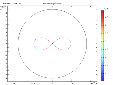
In the Model Builder window, under Study 1: Figure-Eight Configuration click Step 1: Time Dependent.
2
In the Settings window for Time Dependent, locate the Study Settings section.
3
In the Output times text field, type range(0,T1/100,10*T1).
4
From the Tolerance list, choose User controlled.
5
In the Relative tolerance text field, type 1E-10.
6
Locate the Physics and Variables Selection section. Select the Modify model configuration for study step check box.
7
In the tree, select Component 1 (comp1)>Mathematical Particle Tracing (pt)>Release from Grid 4, Component 1 (comp1)>Mathematical Particle Tracing (pt)>Release from Grid 5, and Component 1 (comp1)>Mathematical Particle Tracing (pt)>Release from Grid 6.
8
9
In the Home toolbar, click  Compute.
Results
Figure-Eight Configuration
In the Settings window for 2D Plot Group, type Figure-Eight Configuration in the Label text field.
Particle Trajectories 1
1
In the Model Builder window, expand the Figure-Eight Configuration node, then click Particle Trajectories 1.
2
In the Settings window for Particle Trajectories, locate the Coloring and Style section.
3
Find the Point style subsection. From the Type list, choose Comet tail.
4
Find the Line style subsection. From the Type list, choose Line.
Color Expression 1
1
In the Model Builder window, expand the Particle Trajectories 1 node, then click Color Expression 1.
2
In the Settings window for Color Expression, locate the Coloring and Style section.
3
Click  Change Color Table.
4
In the Color Table dialog box, select Rainbow>RainbowLight in the tree.
5
6
In the Figure-Eight Configuration toolbar, click  Plot. The resulting plot should look like Figure 2.
Animation 1
1
In the Figure-Eight Configuration toolbar, click  Animation and choose Player.
2
In the Settings window for Animation, locate the Frames section.
3
In the Number of frames text field, type 300.
4
Click the  Play button in the Graphics toolbar.
Check Energy Conservation
1
In the Home toolbar, click  Add Plot Group and choose 1D Plot Group.
2
In the Settings window for 1D Plot Group, type Check Energy Conservation in the Label text field.
Global 1
1
Right-click Check Energy Conservation and choose Global.
2
In the Settings window for Global, locate the y-Axis Data section.
3
4
In the Check Energy Conservation toolbar, click  Plot. The resulting plot should look like Figure 3.
Add Study
1
In the Home toolbar, click  Add Study to open the Add Study window.
2
Go to the Add Study window.
3
Find the Studies subsection. In the Select Study tree, select General Studies>Time Dependent.
4
Click Add Study in the window toolbar.
5
In the Home toolbar, click  Add Study to close the Add Study window.
Study 2: Lagrange Configuration
1
In the Model Builder window, click Study 2.
2
In the Settings window for Study, type Study 2: Lagrange Configuration in the Label text field.
Step 1: Time Dependent
1
In the Model Builder window, under Study 2: Lagrange Configuration click Step 1: Time Dependent.
2
In the Settings window for Time Dependent, locate the Study Settings section.
3
In the Output times text field, type range(0,T2/100,10*T2).
4
From the Tolerance list, choose User controlled.
5
In the Relative tolerance text field, type 1E-10.
6
Locate the Physics and Variables Selection section. Select the Modify model configuration for study step check box.
7
In the tree, select Component 1 (comp1)>Mathematical Particle Tracing (pt)>Release from Grid 1, Component 1 (comp1)>Mathematical Particle Tracing (pt)>Release from Grid 2, and Component 1 (comp1)>Mathematical Particle Tracing (pt)>Release from Grid 3.
8
9
In the Home toolbar, click  Compute.
Results
Lagrange Configuration
In the Settings window for 2D Plot Group, type Lagrange Configuration in the Label text field.
Particle Trajectories 1
1
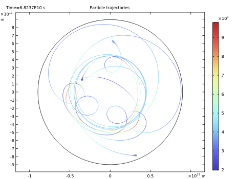
In the Model Builder window, expand the Lagrange Configuration node, then click Particle Trajectories 1.
2
In the Settings window for Particle Trajectories, locate the Coloring and Style section.
3
Find the Line style subsection. From the Type list, choose Line.
4
Find the Point style subsection. From the Type list, choose Comet tail.
Color Expression 1
1
In the Model Builder window, expand the Particle Trajectories 1 node, then click Color Expression 1.
2
In the Settings window for Color Expression, locate the Coloring and Style section.
3
Click  Change Color Table.
4
In the Color Table dialog box, select Rainbow>RainbowLight in the tree.
5
6
In the Lagrange Configuration toolbar, click  Plot. The resulting plot should look similar to Figure 4. However, because the Lagrange configuration is inherently unstable, the exact particle paths may look different. The important feature of this trajectory plot is that the three stars lie at the vertices of a rotating equilateral triangle, but after several orbits the symmetry is visibly broken and the trajectories become more obviously chaotic.
Animation 2
1
In the Lagrange Configuration toolbar, click  Animation and choose Player.
2
In the Settings window for Animation, locate the Frames section.
3
In the Number of frames text field, type 300.
4
Click the  Play button in the Graphics toolbar.