PDF

Shape Optimization of a Shell
Introduction
Shape optimization can be used to alter the geometry of an existing product to improve its performance. You can do that using the Deformed Geometry interface, but you have to decide which shape deformations to allow. It is important to impose some restriction to preserve the mesh quality during the optimization. One approach is to use a Helmholtz filter to introduce a length scale, which (in combination with a maximum displacement parameter) limits the slope of the shape variations. This type of regularized shape optimization can be set up using equation based modeling, but it is also built into the Free Shape Shell feature. This feature differs from the Free Shape Boundary feature in that it can be used on boundaries that are not adjacent to meshed domains.
Model Definition
Shape optimization is often subject to constraints on the geometry deformation, and this model shows how the Free Shape Shell feature can be combined with the Symmetry/Roller feature to restrict edges to move along an imaginary boundary defined by a normal vector. The sides as well as the loaded edges are fixed using the Fixed Edge feature. The initial geometry of the shell is shown in Figure 1. Note that symmetry is exploited so that only half of the shell has to be modeled.
Figure 1: The initial geometry is shown. The load is applied in the y direction on the rightmost edge, while the displacement and rotation is fixed at the leftmost edge of the shell. The shape deformation of this edge is restricted to the xz-plane.
The shell is made of steel and the objective is to maximize its stiffness by deforming it. An initial study is performed to determine a characteristic value for the area and the total elastic strain energy.
The model uses geometric nonlinearity, because the applied load is so large that this is warranted.
Results and Discussion
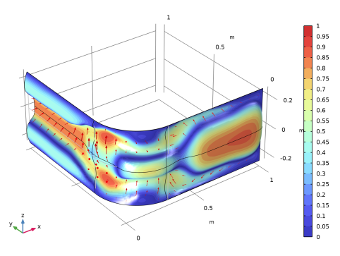
The optimal design is intuitive in the sense that it deforms the shell, so that material is moved away from the midplane, increasing the stiffness of the shell; see Figure 2.
Figure 2: The default shape optimization plot shows the edges of the old geometry in gray together with a surface plot of the relative normal boundary displacement in colors. The actual displacement is shown with red arrows.
By deforming the shell, the optimization is able to reduce the elastic strain energy by 89%. This causes a 9% increase in the surface area.
Notes About the COMSOL Implementation
This model combines the Optimization and Shell interfaces. The shape optimization features are added before the first study is computed, because this automatically sets the correct scales for the shape optimization variables. It is possible to add the shape optimization features after the first study has been computed, but then the first study will no longer converge (the shape optimization variables cannot be disabled).
Application Library path: Optimization_Module/Shape_Optimization/shell_shape_optimization
Modeling Instructions
From the File menu, choose New.
New
In the New window, click  Model Wizard.
Model Wizard
1
In the Model Wizard window, click  3D.
2
In the Select Physics tree, select Structural Mechanics>Shell (shell).
3
Click Add.
4
Click  Study.
5
In the Select Study tree, select General Studies>Stationary.
6
Global Definitions
Parameters 1
1
In the Model Builder window, under Global Definitions click Parameters 1.
2
In the Settings window for Parameters, locate the Parameters section.
3
Geometry 1
Work Plane 1 (wp1)
In the Geometry toolbar, click  Work Plane.
Work Plane 1 (wp1)>Plane Geometry
In the Model Builder window, click Plane Geometry.
Work Plane 1 (wp1)>Square 1 (sq1)
In the Work Plane toolbar, click  Square.
Work Plane 1 (wp1)>Fillet 1 (fil1)
1
In the Work Plane toolbar, click  Fillet.
2
On the object sq1, select Point 1 only.
3
In the Settings window for Fillet, locate the Radius section.
4
In the Radius text field, type 0.3.
Work Plane 1 (wp1)>Convert to Curve 1 (ccur1)
1
In the Work Plane toolbar, click  Conversions and choose Convert to Curve.
2
Edges to Delete
1
In the Work Plane toolbar, click  Selections and choose Box Selection.
2
In the Settings window for Box Selection, type Edges to Delete in the Label text field.
3
Locate the Geometric Entity Level section. From the Level list, choose Boundary.
4
Locate the Box Limits section. In the xw minimum text field, type 0.9.
5
In the yw minimum text field, type 0.9.
Work Plane 1 (wp1)>Delete Entities 1 (del1)
1
Right-click Plane Geometry and choose Delete Entities.
2
In the Settings window for Delete Entities, locate the Entities or Objects to Delete section.
3
From the Selection list, choose Edges to Delete.
Extrude 1 (ext1)
1
In the Model Builder window, right-click Geometry 1 and choose Extrude.
2
In the Settings window for Extrude, locate the Distances section.
3
4
Locate the Selections of Resulting Entities section. Select the Resulting objects selection check box.
5
From the Show in physics list, choose Boundary selection.
6
In the Geometry toolbar, click  Build All.
The geometry should now look like that in Figure 1.
Exterior Edges
1
In the Geometry toolbar, click  Selections and choose Adjacent Selection.
2
In the Settings window for Adjacent Selection, type Exterior Edges in the Label text field.
3
Locate the Input Entities section. From the Geometric entity level list, choose Boundary.
4
Locate the Output Entities section. From the Geometric entity level list, choose Adjacent edges.
5
Locate the Input Entities section. Click  Add.
6
In the Add dialog box, select Extrude 1 in the Input selections list.
7
Symmetry Edge
1
In the Geometry toolbar, click  Selections and choose Box Selection.
2
In the Settings window for Box Selection, locate the Geometric Entity Level section.
3
From the Level list, choose Edge.
4
In the Label text field, type Symmetry Edge.
5
Locate the Box Limits section. In the z maximum text field, type eps.
6
Locate the Output Entities section. From the Include entity if list, choose Entity inside box.
7
In the Geometry toolbar, click  Build All.
The model geometry is now complete.
Add Material
1
In the Home toolbar, click  Add Material to open the Add Material window.
2
Go to the Add Material window.
3
In the tree, select Built-in>Structural steel.
4
Click Add to Component in the window toolbar.
5
In the Home toolbar, click  Add Material to close the Add Material window.
Mesh 1
Mapped 1
1
In the Mesh toolbar, click  Boundary and choose Mapped.
2
In the Settings window for Mapped, locate the Boundary Selection section.
3
From the Selection list, choose All boundaries.
Size
1
In the Model Builder window, click Size.
2
In the Settings window for Size, locate the Element Size section.
3
From the Predefined list, choose Finer.
4
Click to expand the Element Size Parameters section. In the Maximum element size text field, type Lmax.
5
In the Minimum element size text field, type Lmax/2.
6
Click  Build All.
Shell (shell)
Enable weak slit and normal constraints to get the correct gradient from the sensitivity analysis performed during the optimization.
1
In the Model Builder window, under Component 1 (comp1) click Shell (shell).
2
In the Settings window for Shell, click to expand the Fold-Line Settings section.
3
Select the Use weak constraints check box.
4
Click the  Show More Options button in the Model Builder toolbar.
5
In the Show More Options dialog box, select Physics>Advanced Physics Options in the tree.
6
In the tree, select the check box for the node Physics>Advanced Physics Options.
7
8
In the Settings window for Shell, click to expand the Advanced Settings section.
9
From the Normal constraint type list, choose Weak constraint.
Fixed Constraint 1
1
In the Physics toolbar, click  Edges and choose Fixed Constraint.
2
3
In the Settings window for Fixed Constraint, click to expand the Constraint Settings section.
4
Select the Use weak constraints check box.
Edge Load 1
1
In the Physics toolbar, click  Edges and choose Edge Load.
2
3
In the Settings window for Edge Load, locate the Force section.
4
From the Load type list, choose Total force.
5
Specify the Ftot vector as
Symmetry 1
1
In the Physics toolbar, click  Edges and choose Symmetry.
2
In the Settings window for Symmetry, locate the Edge Selection section.
3
From the Selection list, choose Symmetry Edge.
4
Locate the Coordinate System Selection section. From the Coordinate system list, choose Global coordinate system.
5
Locate the Symmetry section. From the Symmetry plane normal list, choose Third axis.
6
Click to expand the Constraint Settings section. Select the Use weak constraints check box.
Component 1 (comp1)
Define the shape optimization problem using the Free Shape Shell, Symmetry/Roller and Fixed Edge features.
Free Shape Shell 1
1
In the Definitions toolbar, click  Optimization and choose Shape Optimization>Free Shape Shell.
2
In the Settings window for Free Shape Shell, locate the Boundary Selection section.
3
From the Selection list, choose All boundaries.
4
Locate the Control Variable Settings section. In the text field, type Lmax.
5
Locate the Filtering section. From the Rmin list, choose Small.
Fixed Edge 1
1
In the Definitions toolbar, click  Optimization and choose Shape Optimization>Fixed Edge.
2
In the Settings window for Fixed Edge, locate the Edge Selection section.
3
From the Selection list, choose Exterior Edges.
Symmetry/Roller 1
1
In the Definitions toolbar, click  Optimization and choose Shape Optimization>Symmetry/Roller.
2
In the Settings window for Symmetry/Roller, locate the Geometric Entity Selection section.
3
From the Geometric entity level list, choose Edge.
4
5
Locate the Prescribed Normal Vector section. Specify the n vector as
Symmetry/Roller 2
1
Right-click Symmetry/Roller 1 and choose Duplicate.
2
In the Settings window for Symmetry/Roller, locate the Geometric Entity Selection section.
3
From the Selection list, choose Symmetry Edge.
4
In the Model Builder window, click Symmetry/Roller 2.
5
Locate the Prescribed Normal Vector section. Specify the n vector as
Study 1
Step 1: Stationary
1
In the Model Builder window, under Study 1 click Step 1: Stationary.
2
In the Settings window for Stationary, locate the Study Settings section.
3
Select the Include geometric nonlinearity check box.
4
Locate the Physics and Variables Selection section. Select the Modify model configuration for study step check box.
5
In the tree, select Component 1 (comp1)>Shape Optimization, Controls material frame.
6
Click  Disable in Solvers.
7
Click  Control Frame Deformation.
The initial design has low stiffness, so the problem becomes highly nonlinear. Use continuation in the load to make a continuous transition from the linear regime.
8
Click to expand the Study Extensions section. Select the Auxiliary sweep check box.
9
10
11
In the Model Builder window, click Study 1.
12
In the Settings window for Study, type Initial Design in the Label text field.
13
In the Home toolbar, click  Compute.
Results
Shape Optimization
In the Model Builder window, under Results right-click Shape Optimization and choose Delete.
Add Study
1
In the Home toolbar, click  Add Study to open the Add Study window.
2
Go to the Add Study window.
3
Find the Studies subsection. In the Select Study tree, select General Studies>Stationary.
4
Click Add Study in the window toolbar.
5
In the Home toolbar, click  Add Study to close the Add Study window.
Study 2
Step 1: Stationary
1
In the Settings window for Stationary, locate the Study Settings section.
2
Select the Include geometric nonlinearity check box.
3
Click to expand the Study Extensions section. Select the Auxiliary sweep check box.
4
5
6
In the Model Builder window, click Study 2.
7
In the Settings window for Study, type Shape Optimization in the Label text field.
Shape Optimization
1
In the Study toolbar, click  Optimization and choose Shape Optimization.
2
In the Settings window for Shape Optimization, locate the Optimization Solver section.
3
Clear the Move limits check box.
4
In the Maximum number of iterations text field, type 25.
5
Click Add Expression in the upper-right corner of the Objective Function section. From the menu, choose Component 1 (comp1)>Shell>Global>comp1.shell.Ws_tot - Total elastic strain energy - J.
Scale the objective with the initial value.
6
Locate the Objective Function section. From the Solution list, choose Use last.
7
From the Objective scaling list, choose Initial solution based.
8
In the Study toolbar, click  Get Initial Value.
Results
Mirror 3D 1
1
In the Model Builder window, expand the Results>Datasets node.
2
Right-click Results>Datasets and choose More 3D Datasets>Mirror 3D.
3
In the Settings window for Mirror 3D, locate the Plane Data section.
4
From the Plane list, choose XY-planes.
5
Locate the Data section. From the Dataset list, choose Shape Optimization/Solution 2 (sol2).
Shape Optimization
1
In the Model Builder window, under Results click Shape Optimization.
2
In the Settings window for 3D Plot Group, locate the Data section.
3
From the Dataset list, choose Mirror 3D 1.
Shape Optimization
Solver Configurations
In the Model Builder window, expand the Shape Optimization>Solver Configurations node.
Solution 2 (sol2)
1
In the Model Builder window, expand the Shape Optimization>Solver Configurations>Solution 2 (sol2)>Optimization Solver 1>Stationary 1>Segregated 1 node.
2
Right-click Optimization and choose Move Up to reduce the computational time.
3
In the Model Builder window, click Merged variables.
4
In the Settings window for Segregated Step, click to expand the Method and Termination section.
5
From the Termination technique list, choose Tolerance to reduce the computational time further.
Shape Optimization
1
In the Model Builder window, click Shape Optimization.
2
In the Settings window for Shape Optimization, locate the Output While Solving section.
3
Select the Plot check box.
4
From the Plot group list, choose Shape Optimization.
5
In the Home toolbar, click  Compute.
Results
Stress, Initial Design
1
In the Model Builder window, under Results click Stress (shell).
2
In the Settings window for 3D Plot Group, type Stress, Initial Design in the Label text field.
Stress, Optimized Design
1
In the Model Builder window, under Results click Stress (shell) 1.
2
In the Settings window for 3D Plot Group, type Stress, Optimized Design in the Label text field.
Shape Optimization
1
In the Model Builder window, click Shape Optimization.
2
In the Settings window for 3D Plot Group, type Shape Optimization in the Label text field.