Optimizing a Flywheel Profile

PDF

Optimizing a Flywheel Profile

Flywheels are designed to store kinetic energy by rotating a mass at high speed. The inertial forces load the flywheel causing structural stress which can destroy the flywheel for high rotational frequencies. This model starts out by computing the moment of inertia, the mass, as well as the stress distribution in a simple disk-shaped flywheel. It then uses shape optimization to increase the moment of inertia without increasing the mass or maximum von Mises stress.

Model Definition

The setup of the Solid Mechanics interface is straightforward, and so is the computation of the total mass and moment of inertia via the Mass Properties feature. The main difficulty with the modeling setup thus relates to the use of gradient based optimization in combination with the maximum von mises stress as a constraint.

The Optimization Problem

The maximum von Mises stress will be approximated with a p-norm (p = 10):

(1)

This is a constraint aggregation strategy that performs well for moderate values of p. Too small values cause a bad approximation of the maximum operator, while too large values cause numerical problems for the optimization solver.

The shape optimization problem is setup using the , , and features, such that the inner and outer radii of the flywheel is fixed, that is, it is the profile of the flywheel that is optimized. The feature is set up with a filter radius only one 3rd of the maximum displacement. This means that the slope of the flywheel profile can be as large as 3, which would normally lead to solver errors, but in this model the initial geometry is well suited for a mapped mesh, which is less prone to inverted elements.

Results and Discussion

Figure 1 shows the optimized and initial flywheel profiles.

Figure 1: The von Mises stress for the initial and optimized flywheel design.

The moment of inertia has increased by 9%, while the maximum von Mises stress has been decreased by 36%.

Optimization_Module/Shape_Optimization/flywheel_profile

Modeling Instructions

From the menu, choose .

In the window, click

.

1

In the window, click

.

2

In the tree, select .

3

4

5

In the tree, select .

6

Global Definitions

Type in the parameters for the initial geometry. Note that we exploit symmetry by only modeling half of the flywheel.

1

In the window, under click .

2

In the window for , locate the section.

3

In the table, enter the following settings:


Name	Expression	Value	Description
r0	1[cm]	0.01 m	Inner flywheel radius
r1	60[cm]	0.6 m	Outer flywheel radius
H0	3[cm]	0.03 m	Initial flywheel thickness
omega	2pi50[rad/s]	314.16 rad/s	Angular velocity
pExp	10	10	P-norm exponent

Rectangle 1 (r1)

1

In the toolbar, click

.

2

In the window for , locate the section.

3

In the text field, type r1-r0.

4

In the text field, type H0.

5

Locate the section. In the text field, type r0.

1

In the toolbar, click

to open the window.

2

Go to the window.

3

In the tree, select .

4

Click in the window toolbar.

5

In the toolbar, click

to close the window.

Solid Mechanics (solid)

Rotating Frame 1

1

In the window, under right-click and choose .

2

In the window for , locate the section.

3

In the Ω text field, type omega.

Symmetry Plane 1

1

In the toolbar, click

and choose .

2

Select Boundary 2 only.

In the toolbar, click

.

1

In the window, click .

2

In the window for , locate the section.

3

From the list, choose .

The feature allows computation of the total mass as well as the moment of inertia, but it is not visible by default.

Mass Properties 1 (mass1)

1

In the window, under right-click and choose .

2

In the window for , locate the section.

3

From the list, choose .

Average 1 (aveop1)

1

In the toolbar, click

and choose .

2

In the window for , locate the section.

3

From the list, choose .

1

In the window, click .

2

In the window for , type Initial Design in the text field.

3

Locate the section. Clear the check box.

4

In the toolbar, click

.

1

In the toolbar, click

.

2

In the window for , type Initial Design in the text field.

Initial Constraints

1

Right-click and choose .

Compute the initial P-norm von Mises stress.

2

In the window for , type Initial Constraints in the text field.

3

Locate the section. In the table, enter the following settings:


Expression	Unit	Description
aveop1(solid.mises^pExp)^(1/pExp)	N/m^2	Average 1

4

In the toolbar, click

.

Global Definitions

1

In the window, under click .

2

In the window for , locate the section.

3

In the table, enter the following settings:


Name	Expression	Value	Description
sigma0	96.2[MPa]	9.62E7 Pa	Initial p-norm stress

Component 1 (comp1)

Set up the shape optimization problem and use the p-norm of the von Mises stress as a constraint.

Free Shape Domain 1

1

In the toolbar, click

and choose .

2

In the window for , locate the section.

3

From the list, choose .

Symmetry/Roller 1

1

In the toolbar, click

and choose .

2

Select Boundaries 1 and 4 only.

Free Shape Boundary 1

1

In the toolbar, click

and choose .

2

Select Boundary 3 only.

3

In the window for , locate the section.

4

In the dmax text field, type 2*H0/3.

5

Locate the section. From the Rmin list, choose .

1

In the window, under right-click and choose .

2

In the window for , locate the section.

3

In the table, enter the following settings:


Name	Expression	Unit	Description
stress_Pnorm	aveop1((solid.mises/sigma0)^pExp)^(1/pExp)		Scaled P-norm of von Mises stress

This P-norm is an approximate max operator, which is compatible with gradient based optimization (a real max operator is not). The p-norm is expected to result in unstable behavior for large p.

1

In the toolbar, click

to open the window.

2

Go to the window.

3

Find the subsection. In the tree, select .

4

Click in the window toolbar.

5

In the toolbar, click

to close the window.

Step 1: Stationary

1

In the window, under click .

2

In the window for , locate the section.

3

In the table, clear the check boxes for and .

Shape Optimization

1

In the window, click .

2

In the window for , type Shape Optimization in the text field.

3

In the toolbar, click

.

1

In the window, expand the node, then click .

2

In the window for , locate the section.

3

From the list, choose .

Shape Optimization

Shape Optimization

1

In the toolbar, click

and choose .

2

In the window for , locate the section.

3

From the list, choose .

4

Click in the upper-right corner of the section. From the menu, choose .

5

Click in the upper-right corner of the section. From the menu, choose .

6

Click in the upper-right corner of the section. From the menu, choose .

Scale the moment of inertia with the initial value. Constrain the volume and stress from above, while maximizing the moment of inertia.

7

Locate the section. From the list, choose .

8

From the list, choose .

9

Locate the section. In the table, enter the following settings:


Expression	Lower bound	Upper bound
comp1.fsd1.relVolume		1
comp1.stress_Pnorm		1

10

Locate the section. Select the check box.

11

From the list, choose .

12

In the toolbar, click

.

The optimization moves mass toward the axis to reduce stress, but this reduces the moment of inertia, so material is also moved to the perimeter of the flywheel. Modify the stress plot to include the initial stress distribution.

1

In the toolbar, click

and choose .

2

In the window for , locate the section.

3

In row , set to 1.

4

In row , set to 0.

5

Click to expand the section. Select the check box.

1

Right-click and choose .

2

In the window for , locate the section.

3

From the list, choose .

1

In the window, under click .

2

In the window for , locate the section.

3

From the list, choose .

4

Click to expand the section. From the list, choose .

5

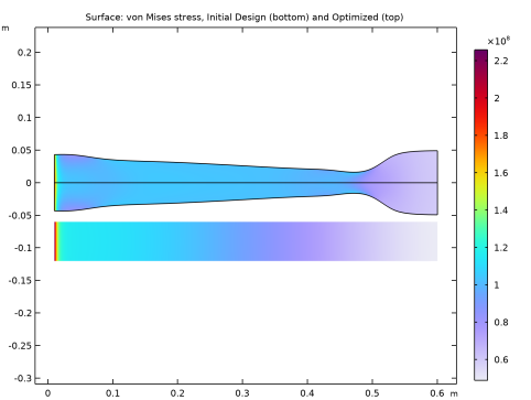
In the text area, type Surface: von Mises stress, Initial Design (bottom) and Optimized (top).

1

In the window, expand the node.

2

Right-click and choose .

1

In the window, expand the node.

2

Right-click and choose .

1

In the window, under click .

2

In the window for , locate the section.

3

From the list, choose .

4

Click to expand the section. From the list, choose .

1

In the window, expand the node, then click .

2

In the window for , locate the section.

3

In the text field, type 0.

4

In the text field, type if(mir1side,1,-1)*-3*H0.

5

Locate the section.

6

Select the check box. In the associated text field, type 1.

7

In the toolbar, click

.

It is clear that the optimization has decreased the maximum stress in the flywheel.