Maximizing the Buckling Load of a Diagonal Brace

PDF

Maximizing the Buckling Load of a Diagonal Brace

Buckling is a common failure mode for slender structures. One can distinguish between tensile and compressive modes, but it is rare to see buckling failure due to a tensile load. The buckling load can normally be increased by adding material, but oftentimes it is possible to achieve the same effect by relocating material.

Model Definition

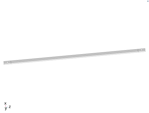
The model studies a structural member, which provides diagonal stiffness in a larger structure. The buckling load of the member is maximized by changing two geometrical parameters, the thickness and the width. The case of a member with a length of 4 m as well as 6 m are studied. The member has a slender geometry as illustrated in Figure 1.

Figure 1: The computational domain is symmetric, but this is not exploited in the model.

The member is made of steel, and the thickness is small, so its structural response can be well characterized using a shell model. The brace is put in compression using a boundary condition with an feature. The initial critical load factor and volume is first calculated and then a second study dealing with the optimization is set up.

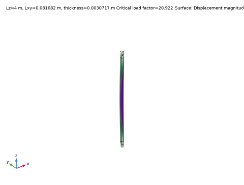
The result of the optimization for a length of 6 m is shown in Figure 2.The Buckling load has been increased by 140%. The bound of the volume constraint is scaled with the brace length, so the 6 m brace is 50% heavier than the 4 m brace. This causes the optimization result for a 4 m brace to have a smaller width and larger thickness than the 6 m brace.

Figure 2: The optimized 6 m member is shown for the 1st buckling mode.

Optimization_Module/Design_Optimization/diagonal_brace_buckling_optimization

Modeling Instructions

From the menu, choose .

In the window, click

.

1

In the window, click

.

2

In the tree, select .

3

4

5

In the tree, select .

6

Global Definitions

1

In the window, under click .

2

In the window for , locate the section.

3

In the table, enter the following settings:


Name	Expression	Value	Description
Lz	6[m]	6 m	Length of brace
Lxy	5[cm]	0.05 m	Brace width
thickness	5[mm]	0.005 m	Brace thickness
Lz1	3*Lxy	0.15 m	Brace end length
Rhole	Lz1/10	0.015 m	Hole radius
Fload	1[kN]	1000 N	Load

1

In the toolbar, click

.

2

In the window for , locate the section.

3

In the text field, type Lxy.

4

In the text field, type Lxy.

5

In the text field, type Lz.

6

Click to expand the section. In the table, enter the following settings:


Layer name	Thickness (m)
Layer 1	Lz1
Layer 1	Lz-2*Lz1

Boundaries to Delete

1

In the toolbar, click

and choose .

2

In the window for , type Boundaries to Delete in the text field.

3

Locate the section. From the list, choose .

4

Locate the section. In the text field, type Lxy*0.1.

5

In the text field, type Lxy*0.1.

Delete Entities 1 (del1)

1

In the window, right-click and choose .

2

In the window for , locate the section.

3

From the list, choose .

4

Locate the section. Select the check box.

Cylinder 1 (cyl1)

1

In the toolbar, click

.

2

In the window for , locate the section.

3

In the text field, type Rhole.

4

In the text field, type Rhole.

5

Locate the section. In the text field, type Lxy/2.

6

In the text field, type -Rhole/2.

7

In the text field, type Lz1/2.

8

Locate the section. From the list, choose .

Cylinder 2 (cyl2)

1

Right-click and choose .

2

In the window for , locate the section.

3

In the text field, type Lz-Lz1/2.

Difference 1 (dif1)

1

In the toolbar, click

and choose .

2

In the window for , locate the section.

3

Find the subsection. Click to select the

toggle button.

4

From the list, choose .

5

Find the subsection. Click to select the

toggle button.

6

Select the objects and only.

7

button in the toolbar.

The geometry should now look like that in Figure 1.

1

In the toolbar, click

and choose .

2

In the window for , type Internal Edges in the text field.

3

Locate the section. From the list, choose .

4

Locate the section. In the text field, type Lz1*0.999.

5

In the text field, type Lz1*1.001.

6

Locate the section. From the list, choose .

Cylinder Selection 1 (cylsel1)

1

In the toolbar, click

and choose .

2

In the window for , locate the section.

3

From the list, choose .

4

Locate the section. In the text field, type Rhole*1.01.

5

Locate the section. In the text field, type Lxy/2.

6

In the text field, type Lz1/2.

7

Locate the section. From the list, choose .

Cylinder Selection 2 (cylsel2)

1

Right-click and choose .

2

In the window for , locate the section.

3

In the text field, type Lz-Lz1/2.

1

In the toolbar, click

to open the window.

2

Go to the window.

3

In the tree, select .

4

Click in the window toolbar.

5

In the toolbar, click

to close the window.

Thickness and Offset 1

1

In the window, under click .

2

In the window for , locate the section.

3

In the d0 text field, type thickness.

Rigid Connector 1

1

In the toolbar, click

and choose .

2

In the window for , locate the section.

3

From the list, choose .

4

Locate the section. Select the check box.

5

Select the check box.

6

Select the check box.

7

Locate the section. From the list, choose .

8

Select the check box.

9

Select the check box.

Rigid Connector 2

1

Right-click and choose .

2

In the window for , locate the section.

3

From the list, choose .

4

Locate the section. Clear the check box.

Applied Force 1

1

In the toolbar, click

and choose .

2

In the window for , locate the section.

3

Specify the F vector as


0	x
0	y
-Fload	z

1

In the toolbar, click

and choose .

2

In the window for , locate the section.

3

From the list, choose .

Right-click and choose .

1

In the toolbar, click

and choose .

2

Select Boundaries 3 and 4 only.

1

Right-click and choose .

2

Select Edge 4 only.

3

In the window for , locate the section.

4

In the text field, type 20.

Free Triangular 1

1

In the toolbar, click

and choose .

2

In the window for , locate the section.

3

From the list, choose .

1

In the window, click .

2

In the window for , locate the section.

3

From the list, choose .

4

.

Mass Properties 1 (mass1)

1

In the window, under right-click and choose .

2

In the window for , locate the section.

3

From the list, choose .

4

From the list, choose .

5

Locate the section. From the list, choose .

1

In the window, click .

2

In the window for , type Initial Design in the text field.

3

In the toolbar, click

.

Mass and Critical Load Factor

1

In the toolbar, click

.

2

In the window for , type Mass and Critical Load Factor in the text field.

Global Evaluation 1

1

Right-click and choose .

2

In the window for , click in the upper-right corner of the section. From the menu, choose .

3

Click in the upper-right corner of the section. From the menu, choose .

4

In the toolbar, click

.

Mode Shape, Initial Design

1

In the window, under click .

2

In the window for , type Mode Shape, Initial Design in the text field.

Global Definitions

1

In the window, under click .

2

In the window for , locate the section.

3

In the table, enter the following settings:


Name	Expression	Value	Description
M0	23.5[kg]	23.5 kg	Initial Mass

1

In the toolbar, click

to open the window.

2

Go to the window.

3

Find the subsection. In the tree, select .

4

Click in the window toolbar.

5

In the toolbar, click

to close the window.

Parametric Sweep

1

In the toolbar, click

.

2

In the window for , locate the section.

3

4

In the table, enter the following settings:


Parameter name	Parameter value list	Parameter unit
Lz (Length of brace)	4 6	m

5

In the window, click .

6

In the window for , type Optimization in the text field.

1

In the toolbar, click

and choose .

2

In the window for , locate the section.

3

From the list, choose .

4

Locate the section. In the table, enter the following settings:


Expression	Description	Evaluate for
abs(comp1.shell.LFcrit)		Linear Buckling

This means that both compressive and tensile failure modes are considered.

5

From the list, choose .

6

From the list, choose .

7

Locate the section. Click

twice.

8

In the table, enter the following settings:


Parameter name	Initial value	Scale	Lower bound	Upper bound
Lxy (Brace width)	5[cm]	5[cm]	1[cm]	20[cm]
thickness (Brace thickness)	5[mm]	5[mm]	1[mm]	20[mm]

9

Click in the upper-right corner of the section. From the menu, choose .

10

Locate the section. In the table, enter the following settings:


Expression	Lower bound	Upper bound	Evaluate for
comp1.mass1.mass/M0		Lz/(6[m])	Linear Buckling

11

In the toolbar, click

.

Mode Shape, Optimization

1

In the window for , type Mode Shape, Optimization in the text field.

2

In the toolbar, click

.

3

button in the toolbar.

Global Evaluation 2

1

In the window, under right-click and choose .

2

In the window for , locate the section.

3

From the list, choose .

4

In the toolbar, click

.

The critical load factor has been improved with a factor of 2 for the 6 m brace.

Create a new plot for the model thumbnail.

1

In the toolbar, click

and choose .

2

In the window for , type Thumbnail in the text field.

3

Locate the section. From the list, choose .

Right-click and choose .

In the window, right-click and choose .

1

In the window, under right-click and choose .

2

In the window for , locate the section.

3

From the list, choose .

4

Click to expand the section. From the list, choose .

1

In the window, right-click and choose .

2

In the window for , locate the section.

3

From the list, choose .

4

Locate the section. In the text field, type 1.

5

Locate the section. From the list, choose .

6

From the list, choose .

1

In the window, right-click and choose .

2

In the window for , locate the section.

3

In the text field, type -0.25.

4

Clear the check box.

5

Right-click and choose .

button in the toolbar.

1

In the window, right-click and choose .

2

In the toolbar, click

.

3

button in the toolbar.