PDF

Bracket — Stress Optimization
with Fatigue Evaluation
Introduction
This model demonstrates how to improve fatigue properties using shape optimization. The fatigue properties are not optimized directly. Instead a heuristic methodology is applied where an approximate value of the maximum stress is minimized subject to constraints on the mass and stiffness.
Model Definition
The model is based on the model Bracket — Fatigue Evaluation in the Fatigue Module Application Library. The initial stiffness as well as fatigue properties can thus be evaluated immediately. The fatigue analysis indicates that failure is likely to occur near some small fillets as illustrated in Figure 1.
Figure 1: The initial fatigue properties.
The Free Shape Domain, Free Shape Boundary, and Symmetry/Roller shape optimization features are used to allow modification of the fillet details, where the maximum stress occurs. COMSOL does not support optimization of the fatigue properties directly, so a heuristic approach is applied. The method is not guaranteed to improve the fatigue properties and therefore it is critical that these are evaluated before and after optimization. The heuristic approach involves using the ap-norm of the von Mises stress as the objective function, ,
For large values of p the objective is a good approximation of the maximum stress, but too large values can cause numerical problems for the optimization solver, so the model uses p = 50.The objective is scaled with the initial value, so (strictly speaking) the maximum stress, σmax, does not play a role; it only serves to prevent unit warnings. COMSOL Multiphysics comes with built-in variables for the volume and the stiffness, so it is easy to specify these constraints. The number of optimization iterations is limited to 20 and an iterative solver is used for the structural mechanics to save computation time.
Results and Discussion
As one might expect the optimization increases the fillet to reduce the maximum stress. This can be seen in Figure 2.
Figure 2: The shape optimization increases the fillet radius at the point of maximum stress.
To verify that the optimization has indeed improved the fatigue properties, a fatigue analysis is performed on the optimized design, and the result can be seen in Figure 3.
Figure 3: The shape optimization has removed the stress concentration at the fillet as compared to the initial design in Figure 2.
Notes About the COMSOL Implementation
The MMA optimization solver is used, but note that the (default) globally convergent behavior is disabled. The Fatigue study step zeros the shape optimization variables, so the model uses the withsol operator to plot the fatigue usage in the deformed frame.
Application Library path: Optimization_Module/Shape_Optimization/bracket_fatigue_optimization
Modeling Instructions
Root
In this example you will start from an existing model from the Fatigue Module.
Application Libraries
1
From the File menu, choose Application Libraries.
2
In the Application Libraries window, select Fatigue Module>Stress Life>bracket_fatigue in the tree.
3
Start by computing the stiffness of the initial design in a new Evaluation Group.
Results
Initial Compliance
1
In the Results toolbar, click  Evaluation Group.
2
In the Settings window for Evaluation Group, type Initial Compliance in the Label text field.
3
Locate the Data section. From the Parameter selection (para) list, choose Last.
Global Evaluation 1
1
Right-click Initial Compliance and choose Global Evaluation.
2
In the Settings window for Global Evaluation, click Add Expression in the upper-right corner of the Expressions section. From the menu, choose Component 1 (comp1)>Solid Mechanics>Global>solid.Ws_tot - Total elastic strain energy - J.
3
In the Initial Compliance toolbar, click  Evaluate.
Global Definitions
Parameters 1
1
In the Model Builder window, under Global Definitions click Parameters 1.
2
In the Settings window for Parameters, locate the Parameters section.
3
Component 1 (comp1)
In the Model Builder window, expand the Component 1 (comp1) node.
Definitions
In the Model Builder window, expand the Component 1 (comp1)>Definitions node.
Free Boundaries
1
In the Model Builder window, expand the Component 1 (comp1)>Definitions>Selections node.
2
Right-click Definitions and choose Selections>Explicit.
3
In the Settings window for Explicit, type Free Boundaries in the Label text field.
4
Locate the Input Entities section. From the Geometric entity level list, choose Boundary.
5
Click  Paste Selection.
6
In the Paste Selection dialog box, type 24, 25, 28, 29, 63, 64, 70, 71 in the Selection text field.
7
Symmetry Boundaries
1
Right-click Free Boundaries and choose Duplicate.
2
In the Settings window for Explicit, type Symmetry Boundaries in the Label text field.
3
Locate the Input Entities section. Click  Clear Selection.
4
Click  Paste Selection.
5
In the Paste Selection dialog box, type 15, 65 in the Selection text field.
6
Free Domains
1
In the Definitions toolbar, click  Adjacent.
2
In the Settings window for Adjacent, locate the Input Entities section.
3
From the Geometric entity level list, choose Boundary.
4
In the Label text field, type Free Domains.
5
Locate the Output Entities section. From the Geometric entity level list, choose Adjacent domains.
6
Locate the Input Entities section. Under Input selections, click  Add.
7
In the Add dialog box, select Free Boundaries in the Input selections list.
8
Average 1 (aveop1)
1
In the Definitions toolbar, click  Nonlocal Couplings and choose Average.
2
In the Settings window for Average, locate the Source Selection section.
3
From the Selection list, choose Free Domains.
Objective Function
1
In the Model Builder window, right-click Definitions and choose Variables.
2
In the Settings window for Variables, type Objective Function in the Label text field.
3
Locate the Variables section. In the table, enter the following settings:
Component 1 (comp1)
Free Shape Domain 1
1
In the Definitions toolbar, click  Optimization and choose Shape Optimization>Free Shape Domain.
2
In the Settings window for Free Shape Domain, locate the Domain Selection section.
3
From the Selection list, choose Free Domains.
Free Shape Boundary 1
1
In the Definitions toolbar, click  Optimization and choose Shape Optimization>Free Shape Boundary.
2
In the Settings window for Free Shape Boundary, locate the Boundary Selection section.
3
From the Selection list, choose Free Boundaries.
The bracket thickness is 8 mm, so we set a maximum displacement that is smaller to avoid inverted elements.
4
Locate the Control Variable Settings section. In the dmax text field, type 3[mm], which corresponds to twice the maximum displacement.
Symmetry/Roller 1
1
In the Definitions toolbar, click  Optimization and choose Shape Optimization>Symmetry/Roller.
2
In the Settings window for Symmetry/Roller, locate the Geometric Entity Selection section.
3
From the Selection list, choose Symmetry Boundaries.
Add Study
1
In the Home toolbar, click  Add Study to open the Add Study window.
2
Go to the Add Study window.
3
Find the Studies subsection. In the Select Study tree, select Empty Study.
4
Click Add Study in the window toolbartwice.
Initial Design
1
In the Model Builder window, click Study 1.
2
In the Settings window for Study, type Initial Design in the Label text field.
Step 1: Stationary
1
In the Model Builder window, expand the Initial Design node.
2
Right-click Initial Design>Step 1: Stationary and choose Copy.
Optimized Design
1
In the Model Builder window, click Study 3.
2
In the Settings window for Study, type Optimized Design in the Label text field.
3
Right-click Optimized Design and choose Paste Stationary.
Shape Optimization
1
In the Study toolbar, click  Optimization and choose Shape Optimization.
2
In the Settings window for Shape Optimization, locate the Optimization Solver section.
3
In the Maximum number of iterations text field, type 15.
4
In the Move limits text field, type 0.2.
5
Click Add Expression in the upper-right corner of the Objective Function section. From the menu, choose Component 1 (comp1)>Definitions>Variables>comp1.obj - Objective function.
Use an if-statement to evaluate the objective for the last solution.
6
Locate the Objective Function section. In the table, enter the following settings:
7
From the Objective scaling list, choose Initial solution based.
8
Click Add Expression in the upper-right corner of the Constraints section. From the menu, choose Component 1 (comp1)>Definitions>Free Shape Domain 1>comp1.fsd1.relVolume - Material volume divided by geometry volume.
9
Click Add Expression in the upper-right corner of the Constraints section. From the menu, choose Component 1 (comp1)>Solid Mechanics>Global>comp1.solid.Ws_tot - Total elastic strain energy - J.
10
Locate the Constraints section. In the table, enter the following settings:
This prevents the optimized design from being heavier or less stiff.
11
In the Study toolbar, click  Get Initial Value.
Results
Applied Loads (solid) 1, Stress (solid) 1
1
In the Model Builder window, under Results, Ctrl-click to select Stress (solid) 1 and Applied Loads (solid) 1.
2
Optimized Design
Solver Configurations
In the Model Builder window, expand the Optimized Design>Solver Configurations node.
Solution 3 (sol3)
1
In the Model Builder window, expand the Optimized Design>Solver Configurations>Solution 3 (sol3) node, then click Optimization Solver 1.
2
In the Settings window for Optimization Solver, locate the Optimization Solver section.
3
Clear the Globally Convergent MMA check boxto save computational time.
4
In the Model Builder window, expand the Optimized Design>Solver Configurations>Solution 3 (sol3)>Optimization Solver 1>Stationary 1>Segregated 1 node, then click Solid Mechanics.
5
In the Settings window for Segregated Step, locate the General section.
6
From the Linear solver list, choose Suggested Iterative Solver (solid)to reduce the computational time further.
Shape Optimization
1
In the Model Builder window, under Optimized Design click Shape Optimization.
2
In the Settings window for Shape Optimization, locate the Output While Solving section.
3
Select the Plot check box.
4
From the Plot group list, choose Shape Optimization.
5
In the Study toolbar, click  Compute.
Initial Fatigue
1
In the Model Builder window, click Study 2.
2
In the Settings window for Study, type Initial Fatigue in the Label text field.
3
In the Model Builder window, expand the Initial Fatigue node.
Parametric Sweep, Step 1: Fatigue
1
In the Model Builder window, under Initial Fatigue, Ctrl-click to select Parametric Sweep and Step 1: Fatigue.
2
Optimized Fatigue
1
In the Model Builder window, click Study 4.
2
In the Settings window for Study, type Optimized Fatigue in the Label text field.
Parametric Sweep
Right-click Optimized Fatigue and choose Paste Multiple Items.
Step 1: Fatigue
1
In the Settings window for Fatigue, locate the Values of Dependent Variables section.
2
Find the Values of variables not solved for subsection. From the Study list, choose Optimized Design, Stationary.
3
In the Study toolbar, click  Compute.
Results
Shape Optimization 1
In the Model Builder window, under Results right-click Shape Optimization 1 and choose Delete.
Cycles to Failure, Optimized
1
In the Model Builder window, under Results click Cycles to Failure (ftg) 1.
2
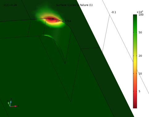
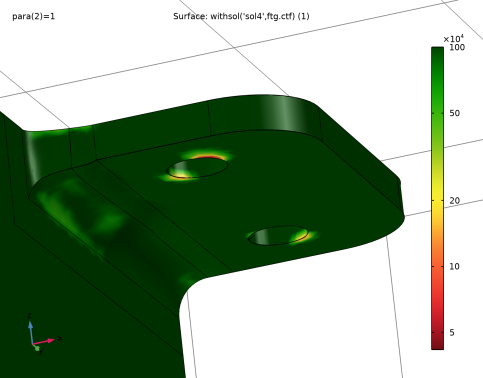
In the Settings window for 3D Plot Group, type Cycles to Failure, Optimized in the Label text field.
The Fatigue study step returns zero for the dependent variables not solved for, so plotting the fatigue usage in the deformed configuration requires the use of the withsol operator.
3
Locate the Data section. From the Dataset list, choose Optimized Design/Solution 3 (sol3).
Surface 1
1
In the Model Builder window, expand the Cycles to Failure, Optimized node, then click Surface 1.
2
In the Settings window for Surface, locate the Expression section.
3
In the Expression text field, type withsol('sol4',ftg.ctf).
Create an Evaluation Group to compare the fatigue properties before and after the optimization.
Fatigue Comparison
1
In the Results toolbar, click  Evaluation Group.
2
In the Settings window for Evaluation Group, type Fatigue Comparison in the Label text field.
3
Locate the Data section. From the Dataset list, choose Initial Fatigue/Solution 2 (sol2).
Surface Minimum 1
1
Right-click Fatigue Comparison and choose Minimum>Surface Minimum.
2
In the Settings window for Surface Minimum, locate the Selection section.
3
From the Selection list, choose Free Boundaries.
4
Click Add Expression in the upper-right corner of the Expressions section. From the menu, choose Component 1 (comp1)>Fatigue>ftg.ctf - Cycles to failure.
Surface Minimum 2
1
Right-click Surface Minimum 1 and choose Duplicate.
2
In the Settings window for Surface Minimum, locate the Data section.
3
From the Dataset list, choose Optimized Fatigue/Solution 4 (sol4).
4
In the Fatigue Comparison toolbar, click  Evaluate.
The fatigue life has been improved by an order of magnitude.
Table
Go to the Table window.
Create a plot for visualizing the shape change using a volumetric representation.
Results
Shape Optimization, Volumetric
1
In the Home toolbar, click  Add Plot Group and choose 3D Plot Group.
2
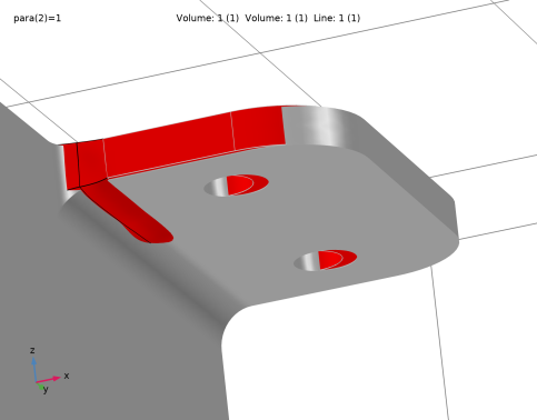
In the Settings window for 3D Plot Group, type Shape Optimization, Volumetric in the Label text field.
3
Locate the Data section. From the Dataset list, choose Optimized Design/Solution 3 (sol3).
Volume 1
1
Right-click Shape Optimization, Volumetric and choose Volume.
2
In the Settings window for Volume, locate the Expression section.
3
In the Expression text field, type 1.
4
Locate the Coloring and Style section. From the Coloring list, choose Uniform.
Volume 2
1
Right-click Volume 1 and choose Duplicate.
2
In the Settings window for Volume, locate the Data section.
3
From the Dataset list, choose Initial Design/Solution 1 (sol1).
4
Locate the Coloring and Style section. From the Color list, choose Gray.
Add a Deformation feature to avoid Z-fighting.
Deformation 1
1
Right-click Volume 2 and choose Deformation.
2
In the Settings window for Deformation, locate the Expression section.
3
In the X component text field, type -Xg*5e-3.
4
In the Y component text field, type -(Yg-0.15)*5e-4.
5
In the Z component text field, type -Zg*5e-4.
6
Locate the Scale section. Select the Scale factor check box.
Line 1
1
In the Model Builder window, right-click Shape Optimization, Volumetric and choose Line.
2
In the Settings window for Line, locate the Data section.
3
From the Dataset list, choose Initial Design/Solution 1 (sol1).
4
Locate the Expression section. In the Expression text field, type 1.
5
Locate the Coloring and Style section. From the Coloring list, choose Uniform.
6
From the Color list, choose Gray.
Shape Optimization, Volumetric
1
In the Model Builder window, click Shape Optimization, Volumetric.
2
In the Settings window for 3D Plot Group, locate the Plot Settings section.
3
From the View list, choose View 3D 2.
4
In the Shape Optimization, Volumetric toolbar, click  Plot.
The optimization increases the fillet radius at the point of maximum stress.
Cycles to Failure, Optimized
1
In the Model Builder window, click Cycles to Failure, Optimized.
2
In the Settings window for 3D Plot Group, locate the Plot Settings section.
3
From the View list, choose View 3D 2.
4
In the Cycles to Failure, Optimized toolbar, click  Plot.
The plot can be compared with the corresponding plot for the initial design.