PDF

Viscoplastic Creep in Solder Joints
Introduction
This example studies viscoplastic creep in solder joints under thermal loading using the Anand viscoplasticity model.
The Anand model is suitable for large, isotropic, viscoplastic deformations in combination with small elastic deformations. The following flow equation takes the stress dependence into account when evaluating strain rate
where is the equivalent viscoplastic strain rate, A is the viscoplastic rate, Q is the activation energy, m is the strain rate sensitivity, ξ is the stress multiplier, R is the ideal gas constant, and T is the absolute temperature.
The internal variable sa is called deformation resistance. A dimensionless counterpart can be defined as sf =sa/ssat , which follows the evolution equation
where
is the saturation value of sf, h0 is the hardening coefficient, a is the exponent for hardening sensitivity, ssat is the coefficient for deformation resistance saturation, and n is the exponent for the deformation resistance sensitivity.
Model Definition
The model geometry is shown in Figure 1. It includes two electronic components (chips) mounted on a circuit board by means of several solder ball joints.
Figure 1: Model geometry.
The solder material is 60Sn40Pb. The circuit board consists of two layers: a thin layer of copper and a thicker layer of FR4 material. The chips are made of silicon. You can find the material and thermal properties for these three materials and for 60Sn40Pb in the material library available in COMSOL Multiphysics.
The nine material parameters needed to apply the Anand model for this solder are available in the literature (Ref. 1). They are summarized in the following table:
Q/R
ssat
sinit
ξ
h0
The structure has initially constant temperature T0 = 20 °C. The heat generation within the chips causes the thermal loading of the structure. At first both components are switched on and operates during 4 h generating a power of 5·107 W/m3. Thereafter, both components are put on stand-by during 2 h, where the power decreases to 1·107 W/m3.
Results and Discussion
When you study the results, bear in mind that the mesh used here is too coarse to produce converged and reliable results for the stresses and strains. The model serves only to display the principal features.
The temperature distribution after 4 h of operation is shown in Figure 2. The temperature is at its maximum and the increase is about 50°C compared to the initial temperature of the circuit board.
Figure 2: Final temperature distribution.
Figure 3 shows change in the deformation resistance through out the operating time.
Figure 3: Evolution of the deformation resistance.
The development of elastic and inelastic strains at a point in a solder joint is shown in Figure 4. An intensive plastic flow appears after about 40 s of the loading, and inelastic strains dominates after about 5 min. The smooth transition at the beginning of the load history and after 4 h is partly affected by the time-dependent hardening behavior and partly affected by the smooth transition in the power load function, where a Heaviside step is replaced with a smooth ramping over a 0.1 h period.
Figure 4: Shear strains in the most critical point.
In a model with creep or viscoplasticity, you can choose to compute also the dissipated energy, as is shown in this example. This quantity is used in several fatigue evaluation criteria when designing against thermal fatigue in electronic components. In Figure 5 the dissipated energy as function of time is shown for the same point as the graphs above.
Figure 5: Viscoplastic dissipation density.
Notes About the COMSOL Implementation
In order to keep the model size down, the mesh is rather coarse (see Figure 6). The results in the solder balls are not accurate enough for making quantitative predictions. In reality, the best approach would probably be to first run a model of this type to find out which solder ball has the largest strains. In a second analysis, you can then analyze a model where an individual solder ball has an improved resolution.
.
Figure 6: Meshed geometry.
Reference
1. Z.N. Cheng, G.Z. Wang, L. Chen, J. Wilde, and K. Becker, “Viscoplastic Anand Model for Solder Alloys and its Application,” Soldering & Surface Mount Technology, vol. 12, no. 2, pp. 31–36, 2000.
Application Library path: Nonlinear_Structural_Materials_Module/Viscoplasticity/viscoplastic_solder_joints
Modeling Instructions
From the File menu, choose New.
New
In the New window, click  Model Wizard.
Model Wizard
1
In the Model Wizard window, click  3D.
2
In the Select Physics tree, select Structural Mechanics>Thermal-Structure Interaction>Thermal Stress, Solid.
3
Click Add.
4
Click  Study.
5
In the Select Study tree, select General Studies>Time Dependent.
6
Global Definitions
Parameters 1
1
In the Model Builder window, under Global Definitions click Parameters 1.
2
In the Settings window for Parameters, locate the Parameters section.
3
Analytic 1 (an1)
1
In the Home toolbar, click  Functions and choose Global>Analytic.
2
In the Settings window for Analytic, type power in the Function name text field.
3
Locate the Definition section. In the Expression text field, type (flc2hs(x-0.1,0.1)*50)-flc2hs(x-(4.1),0.1)*40.
4
Locate the Units section. In the table, enter the following settings:
5
In the Function text field, type MW/m^3.
Geometry 1
Import 1 (imp1)
1
In the Home toolbar, click  Import.
2
In the Settings window for Import, locate the Import section.
3
Click  Browse.
4
5
Click  Import.
Form Union (fin)
In the Home toolbar, click  Build All.
Definitions
FR4
1
In the Definitions toolbar, click  Explicit.
2
In the Settings window for Explicit, type FR4 in the Label text field.
3
Copper
1
In the Definitions toolbar, click  Explicit.
2
In the Settings window for Explicit, type Copper in the Label text field.
3
Silicon
1
In the Definitions toolbar, click  Explicit.
2
In the Settings window for Explicit, type Silicon in the Label text field.
3
Solder
1
In the Definitions toolbar, click  Explicit.
2
In the Settings window for Explicit, type Solder in the Label text field.
3
Locate the Input Entities section. Select the All domains check box.
4
You can do this by first copying the text ’4-23 and 25-40’ and then clicking the Paste Selection button next to the Selection box or clicking in the box and pressing Ctrl+V.
Solder_face
1
Right-click Solder and choose Duplicate.
2
In the Settings window for Explicit, type Solder_face in the Label text field.
3
Locate the Output Entities section. From the Output entities list, choose Adjacent boundaries.
Symmetry Boundaries
1
In the Definitions toolbar, click  Explicit.
2
In the Settings window for Explicit, type Symmetry Boundaries in the Label text field.
3
Locate the Input Entities section. From the Geometric entity level list, choose Boundary.
4
Symmetry Complement
1
In the Definitions toolbar, click  Complement.
2
In the Settings window for Complement, type Symmetry Complement in the Label text field.
3
Locate the Geometric Entity Level section. From the Level list, choose Boundary.
4
Locate the Input Entities section. Under Selections to invert, click  Add.
5
In the Add dialog box, select Symmetry Boundaries in the Selections to invert list.
6
Multiphysics
Thermal Expansion 1 (te1)
1
In the Model Builder window, under Component 1 (comp1)>Multiphysics click Thermal Expansion 1 (te1).
2
In the Settings window for Thermal Expansion, locate the Model Input section.
3
Click  Go to Source for Volume reference temperature.
Global Definitions
Default Model Inputs
1
In the Model Builder window, under Global Definitions click Default Model Inputs.
2
In the Settings window for Default Model Inputs, locate the Browse Model Inputs section.
3
Find the Expression for remaining selection subsection. In the Volume reference temperature text field, type T0.
Solid Mechanics (solid)
Linear Elastic Material 1
In the Model Builder window, under Component 1 (comp1)>Solid Mechanics (solid) click Linear Elastic Material 1.
Viscoplasticity 1
1
In the Physics toolbar, click  Attributes and choose Viscoplasticity.
2
In the Settings window for Viscoplasticity, locate the Domain Selection section.
3
From the Selection list, choose Solder.
Add an equation for integrating the dissipated viscoplastic energy.
4
Click the  Show More Options button in the Model Builder toolbar.
5
In the Show More Options dialog box, in the tree, select the check box for the node Physics>Advanced Physics Options.
6
Linear Elastic Material 1
1
In the Model Builder window, click Linear Elastic Material 1.
2
In the Settings window for Linear Elastic Material, click to expand the Energy Dissipation section.
3
Select the Calculate dissipated energy check box.
Symmetry 1
1
In the Physics toolbar, click  Boundaries and choose Symmetry.
2
In the Settings window for Symmetry, locate the Boundary Selection section.
3
From the Selection list, choose Symmetry Boundaries.
Prescribed Displacement 1
1
In the Physics toolbar, click  Points and choose Prescribed Displacement.
2
3
In the Settings window for Prescribed Displacement, locate the Prescribed Displacement section.
4
Select the Prescribed in z direction check box.
Heat Transfer in Solids (ht)
Initial Values 1
1
In the Model Builder window, under Component 1 (comp1)>Heat Transfer in Solids (ht) click Initial Values 1.
2
In the Settings window for Initial Values, locate the Initial Values section.
3
In the T text field, type T0.
Symmetry 1
1
In the Physics toolbar, click  Boundaries and choose Symmetry.
2
In the Settings window for Symmetry, locate the Boundary Selection section.
3
From the Selection list, choose Symmetry Boundaries.
Heat Source 1
1
In the Physics toolbar, click  Domains and choose Heat Source.
2
In the Settings window for Heat Source, locate the Domain Selection section.
3
From the Selection list, choose Silicon.
4
Locate the Heat Source section. In the Q0 text field, type power(t).
Heat Flux 1
1
In the Physics toolbar, click  Boundaries and choose Heat Flux.
Apply a heat flux on all exterior boundaries except those with prescribed symmetry.
2
In the Settings window for Heat Flux, locate the Boundary Selection section.
3
From the Selection list, choose Symmetry Complement.
4
Locate the Heat Flux section. From the Flux type list, choose Convective heat flux.
5
In the h text field, type 10.
6
In the Text text field, type T0.
Add Material
1
In the Home toolbar, click  Add Material to open the Add Material window.
2
Go to the Add Material window.
3
In the tree, select Built-in>FR4 (Circuit Board).
4
Right-click and choose Add to Global Materials.
5
In the tree, select Built-in>Copper.
6
Right-click and choose Add to Global Materials.
7
In the tree, select Built-in>Silicon.
8
Right-click and choose Add to Global Materials.
9
In the tree, select Built-in>Solder, 60Sn-40Pb.
10
Right-click and choose Add to Global Materials.
11
In the Home toolbar, click  Add Material to close the Add Material window.
Materials
Material Link 1 (matlnk1)
1
In the Model Builder window, under Component 1 (comp1) right-click Materials and choose More Materials>Material Link.
2
In the Settings window for Material Link, locate the Geometric Entity Selection section.
3
From the Selection list, choose FR4.
4
Click to expand the Appearance section. From the Material type list, choose PCB (green).
5
In the Graphics window toolbar, clicknext to  Colors, then choose Show Material Color and Texture.
Material Link 2 (matlnk2)
1
Right-click Materials and choose More Materials>Material Link.
2
In the Settings window for Material Link, locate the Geometric Entity Selection section.
3
From the Selection list, choose Copper.
4
Locate the Link Settings section. From the Material list, choose Copper (mat2).
5
Click to expand the Appearance section. From the Material type list, choose Copper.
Material Link 3 (matlnk3)
1
Right-click Materials and choose More Materials>Material Link.
2
In the Settings window for Material Link, locate the Geometric Entity Selection section.
3
From the Selection list, choose Silicon.
4
Locate the Link Settings section. From the Material list, choose Silicon (mat3).
5
Click to expand the Appearance section. From the Color list, choose Black.
Material Link 4 (matlnk4)
1
Right-click Materials and choose More Materials>Material Link.
2
In the Settings window for Material Link, locate the Geometric Entity Selection section.
3
From the Selection list, choose Solder.
4
Locate the Link Settings section. From the Material list, choose Solder, 60Sn-40Pb (mat4).
5
Click to expand the Appearance section. From the Material type list, choose Steel.
Global Definitions
Solder, 60Sn-40Pb (mat4)
1
In the Model Builder window, under Global Definitions>Materials click Solder, 60Sn-40Pb (mat4).
2
In the Settings window for Material, locate the Material Properties section.
3
In the Material properties tree, select Solid Mechanics>Viscoplastic Material>Anand Viscoplasticity.
4
Click  Add to Material.
5
Locate the Material Contents section. In the table, enter the following settings:
Ω·m
Mesh 1
1
In the Model Builder window, under Component 1 (comp1) click Mesh 1.
2
In the Settings window for Mesh, locate the Sequence Type section.
3
From the list, choose User-controlled mesh.
Free Tetrahedral 1
1
In the Model Builder window, under Component 1 (comp1)>Mesh 1 click Free Tetrahedral 1.
2
In the Settings window for Free Tetrahedral, locate the Domain Selection section.
3
From the Geometric entity level list, choose Domain.
4
From the Selection list, choose Solder.
Size
1
In the Model Builder window, click Size.
2
In the Settings window for Size, locate the Element Size section.
3
From the Predefined list, choose Fine.
Free Tetrahedral 1
1
In the Model Builder window, right-click Free Tetrahedral 1 and choose Build All.
2
Click the  Wireframe Rendering button in the Graphics toolbar to see the meshed domains.
Free Triangular 1
1
In the Mesh toolbar, click  Boundary and choose Free Triangular.
2
3
In the Settings window for Free Triangular, click  Build All.
Swept 1
1
In the Mesh toolbar, click  Swept.
2
In the Settings window for Swept, locate the Domain Selection section.
3
From the Geometric entity level list, choose Domain.
4
From the Selection list, choose Copper.
5
Click  Build All.
Free Tetrahedral 2
1
In the Mesh toolbar, click  Free Tetrahedral.
2
In the Settings window for Free Tetrahedral, click  Build All.
3
Click the  Wireframe Rendering button in the Graphics toolbar.
Study 1
Step 1: Time Dependent
The coupling only applies from Heat Transfer in Solids to Solid Mechanics. Solve Heat Transfer in Solids in a first time-dependent step and then Solid Mechanics in a second time-dependent step.
1
In the Model Builder window, under Study 1 click Step 1: Time Dependent.
2
In the Settings window for Time Dependent, locate the Study Settings section.
3
From the Time unit list, choose h.
4
In the Output times text field, type 0 0.005 range(0.025,0.025,0.5) range(0.75,0.25,3.75) 3.975 4+{range(0,0.025,0.5) range(0.75,0.25,2)}.
5
Locate the Physics and Variables Selection section. In the table, clear the Solve for check box for Solid Mechanics (solid).
Time Dependent 2
1
In the Study toolbar, click  Study Steps and choose Time Dependent>Time Dependent.
2
In the Settings window for Time Dependent, locate the Study Settings section.
3
From the Time unit list, choose h.
4
In the Output times text field, type 0 0.005 range(0.025,0.025,0.5) range(0.75,0.25,3.75) 3.975 4+{range(0,0.025,0.5) range(0.75,0.25,2)}.
5
Locate the Physics and Variables Selection section. In the table, clear the Solve for check box for Heat Transfer in Solids (ht).
6
Click to expand the Values of Dependent Variables section. Find the Values of variables not solved for subsection. From the Settings list, choose User controlled.
7
From the Method list, choose Solution.
8
From the Study list, choose Study 1, Time Dependent.
9
From the Selection list, choose Automatic (all solutions).
Solution 1 (sol1)
1
In the Study toolbar, click  Show Default Solver.
In cases where time derivatives are not important as results, the file size can be significantly reduced by not storing these variables.
2
In the Model Builder window, expand the Solution 1 (sol1) node, then click Time-Dependent Solver 1.
3
In the Settings window for Time-Dependent Solver, click to expand the Output section.
4
Clear the Store time derivatives check box.
5
Click to expand the Time Stepping section. From the Steps taken by solver list, choose Strict.
6
In the Model Builder window, expand the Study 1>Solver Configurations>Solution 1 (sol1)>Dependent Variables 2 node, then click Viscoplastic dissipation density (comp1.solid.Wvp).
7
In the Settings window for Field, locate the Scaling section.
8
From the Method list, choose Manual.
9
In the Scale text field, type 1e5.
Setting an accurate scale for the viscoplastic energy dissipation will improve the automatic time stepping.
10
In the Model Builder window, under Study 1>Solver Configurations>Solution 1 (sol1) click Time-Dependent Solver 2.
11
In the Settings window for Time-Dependent Solver, locate the Output section.
12
Clear the Store time derivatives check box.
13
Locate the Time Stepping section. From the Steps taken by solver list, choose Strict.
14
Find the Algebraic variable settings subsection. From the Error estimation list, choose Exclude algebraic.
The viscoplastic energy dissipation is not part of problem to be solved, but rather a result quantity to be computed. Set the solver to segregated and place the variable in its own segregated step. Changing this is not necessary, but it will reduce the memory requirements somewhat.
15
Right-click Study 1>Solver Configurations>Solution 1 (sol1)>Time-Dependent Solver 2 and choose Segregated.
16
In the Settings window for Segregated, locate the General section.
17
From the Termination technique list, choose Iterations.
18
In the Model Builder window, expand the Study 1>Solver Configurations>Solution 1 (sol1)>Time-Dependent Solver 2>Segregated 1 node, then click Segregated Step.
19
In the Settings window for Segregated Step, type Displacement Field in the Label text field.
20
Locate the General section. In the Variables list, select Viscoplastic dissipation density (comp1.solid.Wvp).
21
Under Variables, click  Delete.
22
Click to expand the Method and Termination section. From the Termination technique list, choose Tolerance.
23
In the Tolerance factor text field, type 1.
24
In the Model Builder window, under Study 1>Solver Configurations>Solution 1 (sol1)>Time-Dependent Solver 2 right-click Segregated 1 and choose Segregated Step.
25
In the Settings window for Segregated Step, type Energy Dissipation in the Label text field.
26
Locate the Method and Termination section. From the Termination technique list, choose Tolerance.
27
In the Tolerance factor text field, type 1.
28
Locate the General section. Under Variables, click  Add.
29
In the Add dialog box, select Viscoplastic dissipation density (comp1.solid.Wvp) in the Variables list.
30
31
In the Study toolbar, click  Compute.
Results
Temperature (ht)
1
In the Model Builder window, under Results click Temperature (ht).
2
In the Settings window for 3D Plot Group, locate the Data section.
3
From the Time (h) list, choose 1.
Surface
1
In the Model Builder window, expand the Temperature (ht) node, then click Surface.
2
In the Settings window for Surface, locate the Expression section.
3
From the Unit list, choose degC.
4
In the Temperature (ht) toolbar, click  Plot.
Display the deformation resistance history.
Deformation Resistance History
1
In the Home toolbar, click  Add Plot Group and choose 1D Plot Group.
2
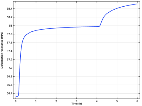
In the Settings window for 1D Plot Group, type Deformation Resistance History in the Label text field.
3
Click to expand the Title section. From the Title type list, choose None.
Point Graph 1
1
Right-click Deformation Resistance History and choose Point Graph.
2
3
In the Settings window for Point Graph, locate the y-Axis Data section.
4
In the Expression text field, type solid.saGp.
5
From the Unit list, choose MPa.
6
Click to expand the Coloring and Style section. From the Width list, choose 2.
7
In the Deformation Resistance History toolbar, click  Plot.
Display the strain history.
Strain History
1
In the Home toolbar, click  Add Plot Group and choose 1D Plot Group.
2
In the Settings window for 1D Plot Group, type Strain History in the Label text field.
Point Graph 1
1
Right-click Strain History and choose Point Graph.
2
3
In the Settings window for Point Graph, locate the y-Axis Data section.
4
In the Expression text field, type solid.gpeval(solid.el13).
5
Locate the Coloring and Style section. From the Width list, choose 2.
6
Click to expand the Legends section. Select the Show legends check box.
7
From the Legends list, choose Manual.
8
Point Graph 2
1
Right-click Point Graph 1 and choose Duplicate.
2
In the Settings window for Point Graph, locate the y-Axis Data section.
3
In the Expression text field, type solid.gpeval(solid.evpl13).
4
Locate the Legends section. In the table, enter the following settings:
Point Graph 3
1
Right-click Point Graph 2 and choose Duplicate.
2
In the Settings window for Point Graph, locate the y-Axis Data section.
3
In the Expression text field, type solid.gpeval(solid.el13-solid.evpl13).
4
Locate the Legends section. In the table, enter the following settings:
Strain History
1
In the Model Builder window, click Strain History.
2
In the Settings window for 1D Plot Group, locate the Plot Settings section.
3
Select the y-axis label check box. In the associated text field, type Shear strain, xz-component.
4
Locate the Title section. From the Title type list, choose None.
5
Locate the Legend section. From the Layout list, choose Outside graph axis area.
6
From the Position list, choose Bottom.
7
In the Strain History toolbar, click  Plot.
Display the dissipation history.
Dissipation History
1
In the Model Builder window, right-click Deformation Resistance History and choose Duplicate.
2
In the Settings window for 1D Plot Group, type Dissipation History in the Label text field.
Point Graph 1
1
In the Model Builder window, expand the Dissipation History node, then click Point Graph 1.
2
In the Settings window for Point Graph, click Replace Expression in the upper-right corner of the y-Axis Data section. From the menu, choose Component 1 (comp1)>Solid Mechanics>Energy and power>solid.WvpGp - Viscoplastic dissipation density - J/m³.
3
Locate the y-Axis Data section. From the Unit list, choose kJ/m^3.
Dissipation History
1
In the Model Builder window, click Dissipation History.
2
In the Dissipation History toolbar, click  Plot.
Finally, display the temperature history.
Temperature History
1
Right-click Dissipation History and choose Duplicate.
2
In the Settings window for 1D Plot Group, type Temperature History in the Label text field.
Point Graph 1
1
In the Model Builder window, expand the Temperature History node, then click Point Graph 1.
2
In the Settings window for Point Graph, click Replace Expression in the upper-right corner of the y-Axis Data section. From the menu, choose Component 1 (comp1)>Heat Transfer in Solids>Temperature>T - Temperature - K.
3
Locate the y-Axis Data section. From the Unit list, choose degC.
4
In the Temperature History toolbar, click  Plot.