You are viewing the documentation for an older COMSOL version. The latest version is available here.
PDF

Submodeling with Plasticity
Introduction
Submodeling is a powerful technique for computing accurate local results in large structures. The basic idea is that a small detailed model is analyzed, driven by boundary conditions that are given by the results from a global model.
In this example, it is shown how you can incorporate nonlinearities in a submodel. The source of the nonlinearity is plasticity, but the same approach can be used also for other cases. The only important thing is the fundamental assumption that the properties of the submodel are such that its stiffness does not differ significantly from what is computed from the same volume of material in the global model.
If the material would have an explicit time dependency, as would be the case for creep, then the submodel would have to be analyzed in time domain.
The global model can be either considered as linear or be analyzed under the same nonlinear conditions as the submodel. A nonlinear analysis would provide somewhat better boundary conditions for the submodel, but may be computationally too expensive for a large structure.
This example is an extension of the model Submodeling Analysis of a Shaft in the COMSOL Multiphysics Application Library, where the general submodeling technique is discussed in more detail.
Model Definition
The geometry consists of a shaft with a sudden change in diameter. At the location of the diameter change, there is a fillet with a small radius where stress concentrations will appear. There is also a central hole through the shaft. The geometry and mesh are shown in Figure 1.
The shaft is fixed at the thick end. On the thin end, a tensile force of 2500 N and a shear force of 900 N are applied.
The material is steel, with Young’s modulus 200 GPa and Poisson’s ratio 0.3.
The yield stress is 350 MPa, and a linear hardening with tangent modulus 1.045 GPa is assumed.
Figure 1: The full model.
As submodel, a region around the fillet at the side giving the highest stress is chosen.
The geometry and mesh of the submodel are shown in Figure 2.
Figure 2: The submodel.
Results and Discussion
In the original linear model, the computed maximum von Mises stress is 466 MPa. This is well above the yield limit of 350 MPa. A plot of the stress contour for the yield limit, Figure 3, shows that the yield stress is exceeded only in a smaller region in the fillet. This indicates that it can be possible to apply the submodeling technique to determine the stress and strain state accurately. Since only a small volume of the material will yield, the stiffness of the component should not be affected too much.
Figure 3: Stress distribution in the linear analysis. The contour shows the yield limit.
In Figure 4, the stress distribution after the full nonlinear analysis is shown. The peak stress is now 351 MPa. There is only a small amount of hardening. In the same figure, the actual size of the plastic region is shown, together with the previous estimate from the nonlinear analysis.
Figure 4: Von Mises equivalent stress at full load in the elastoplastic analysis. The yellow contour shows where the yield stress was exceeded in the elastic analysis while the cyan contour shows the same limit in the elastoplastic analysis.
In Figure 5, the equivalent plastic strain field is shown. As can be seen, the plastic zone does not penetrate very deep from the surface of the fillet. This also serves as a verification of the assumption that the introduction of the elastoplastic material model should not affect the overall stiffness significantly.
The maximum plastic strain is about 0.08 %.
It should be noted that even with mesh in the submodel, the plasticity is essentially confined to the outermost layer of elements.
Figure 5: Equivalent plastic strain in the submodel.
As another verification of the validity of the approach is to evaluate the reaction force in the Y-direction for the cut in the thin part of the shaft for all steps in the auxiliary sweep. When normalized by the applied shear load, the value should ideally be constant, and equal to 1. In Figure 6, the result is shown. In the linear regime, the value is 0.990. This can be interpreted as that the submodel actually is 1.0% more compliant than the global model. At full load, the normalized reaction force has decreased to 0.983. The force applied to the submodel is thus about 1.7% too small, which is probably still acceptable.
Figure 6: The normalized cut reaction force as function of the load multiplier.
Notes About the COMSOL Implementation
When a study that either contains an auxiliary sweep, or is time dependent, references results from a previous study, it is important that correct values can be retrieved. This means that the same parameter must be used in both studies.
In time domain, the built-in time parameter (t) is used. In an auxiliary sweep, you must select the same parameter to represent the loading in both studies. The parameter values that are used can however differ. When values are not matching, the results from the previous study are interpolated. Thus, it is a minimum requirement that the range of the loading parameter in the previous study is at least as large as in the one referencing it.
In this example, the first (full model) study is linear. Still, in order for results to be interpolated, a formal auxiliary sweep with two parameter values is required.
In the settings for the second study step, you need to make the appropriate settings under Values of variables not solved for:
Settings: User Controlled
Method: Solution
Study: The global model study
Parameter value: Automatic (all solutions)
If, instead of a linear analysis, you would like to incorporate plasticity also in the global model, you only need to make two changes:
Add a Plasticity node under Linear Elastic Material in the global model.
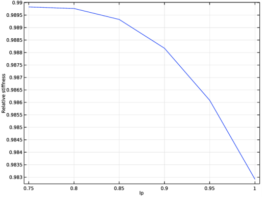
Change the range of the auxiliary sweep in the Full Model study to be, for example range(0.75,0.05,1).
Application Library path: Nonlinear_Structural_Materials_Module/Plasticity/shaft_submodeling_plasticity
Modeling Instructions
Root
Start by opening the existing linear model.
Application Libraries
1
From the File menu, choose Application Libraries.
2
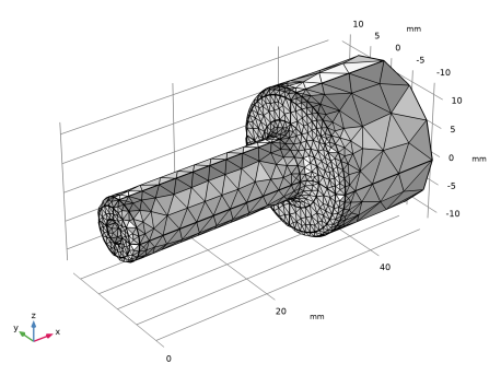
In the Application Libraries window, select COMSOL Multiphysics>Structural Mechanics>shaft_submodeling in the tree.
3
Add a contour indicating the region where the yield stress is exceeded.
Results
Stress - Submodel
1
In the Model Builder window, under Results click Stress - Submodel.
2
In the Settings window for 3D Plot Group, click to expand the Title section.
3
From the Title type list, choose None.
Contour 1
1
Right-click Stress - Submodel and choose Contour.
2
In the Settings window for Contour, locate the Expression section.
3
In the Expression text field, type solid2.misesGp/material.ElastoplasticModel.sigmags.
4
Locate the Levels section. From the Entry method list, choose Levels.
5
In the Levels text field, type 1.
6
Locate the Coloring and Style section. Clear the Color legend check box.
7
From the Coloring list, choose Uniform.
8
From the Color list, choose Cyan.
Deformation
1
In the Model Builder window, expand the Results>Stress - Submodel>Volume 1 node.
2
Right-click Deformation and choose Copy.
Deformation
In the Model Builder window, right-click Contour 1 and choose Paste Deformation.
Contour 1
1
In the Settings window for Contour, click to expand the Inherit Style section.
2
Clear the Color check box.
3
Clear the Color and data range check box.
4
Clear the Transparency check box.
5
Clear the Tube radius scale factor check box.
6
From the Plot list, choose Volume 1.
7
Click the  Show Grid button in the Graphics toolbar.
8
In the Stress - Submodel toolbar, click  Plot.
9
Click the  Zoom Extents button in the Graphics toolbar.
Add a parameter for scaling the load.
Global Definitions
Parameters 1
1
In the Model Builder window, under Global Definitions click Parameters 1.
2
In the Settings window for Parameters, locate the Parameters section.
3
Full Model (comp1)
In the Model Builder window, expand the Full Model (comp1) node.
Solid Mechanics (solid)
Boundary Load 1
1
In the Model Builder window, expand the Full Model (comp1)>Solid Mechanics (solid) node, then click Boundary Load 1.
2
In the Settings window for Boundary Load, locate the Force section.
3
Specify the Ftot vector as
Formally, the linear global model study must also contain an auxiliary sweep. The values of the sweep parameter are not important, as long as the range that will be used in the submodel is covered.
Full Model
Step 1: Stationary
1
In the Model Builder window, expand the Full Model node, then click Step 1: Stationary.
2
In the Settings window for Stationary, click to expand the Study Extensions section.
3
Select the Auxiliary sweep check box.
4
5
6
In the Home toolbar, click  Compute.
Results
Stress - Full Model
Add plasticity to the submodel.
Submodel (comp2)
In the Model Builder window, expand the Submodel (comp2) node.
Solid Mechanics 2 (solid2)
Linear Elastic Material 1
In the Model Builder window, expand the Submodel (comp2)>Solid Mechanics 2 (solid2) node, then click Linear Elastic Material 1.
Plasticity 1
In the Physics toolbar, click  Attributes and choose Plasticity.
Add an auxiliary sweep, where the first load level is still in the linear regime. In this case, this is 75% of the full load.
Submodel
Step 1: Stationary
1
In the Model Builder window, expand the Submodel node, then click Step 1: Stationary.
2
In the Settings window for Stationary, locate the Study Extensions section.
3
Select the Auxiliary sweep check box.
4
5
6
Click to expand the Values of Dependent Variables section. Find the Values of variables not solved for subsection. From the Parameter value (lp) list, choose Automatic (all solutions).
7
In the Home toolbar, click  Compute.
Compare the calculated plastic region with the one estimated from the elastic results.
Results
Contour 2
1
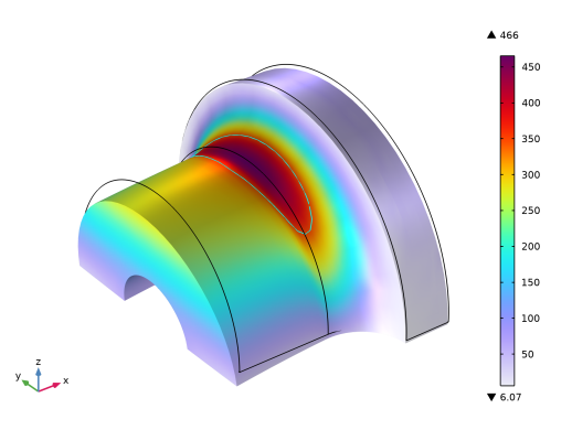
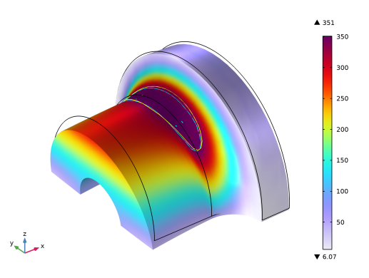
In the Model Builder window, under Results>Stress - Submodel right-click Contour 1 and choose Duplicate.
2
In the Settings window for Contour, locate the Data section.
3
From the Dataset list, choose Submodel/Solution 2 (3) (sol2).
4
From the Parameter value (lp) list, choose 0.75.
5
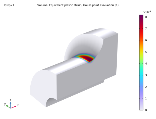
Locate the Expression section. In the Expression text field, type solid2.misesGp/material.ElastoplasticModel.sigmags/0.75.
6
Locate the Coloring and Style section. From the Color list, choose Yellow.
7
In the Stress - Submodel toolbar, click  Plot.
Plastic Strain
1
In the Home toolbar, click  Add Plot Group and choose 3D Plot Group.
2
In the Settings window for 3D Plot Group, type Plastic Strain in the Label text field.
3
Locate the Data section. From the Dataset list, choose Submodel/Solution 2 (3) (sol2).
4
Click  Plot Last.
Volume 1
1
Right-click Plastic Strain and choose Volume.
2
In the Settings window for Volume, locate the Expression section.
3
In the Expression text field, type solid2.epeGp.
4
Locate the Coloring and Style section. Click  Change Color Table.
5
In the Color Table dialog box, select Rainbow>Prism in the tree.
6
Filter 1
1
Right-click Volume 1 and choose Filter.
2
In the Settings window for Filter, locate the Element Selection section.
3
In the Logical expression for inclusion text field, type Y>-0.0001.
4
From the Element nodes to fulfill expression list, choose All.
Plastic Strain
1
In the Model Builder window, under Results click Plastic Strain.
2
In the Settings window for 3D Plot Group, locate the Plot Settings section.
3
Clear the Plot dataset edges check box.
Volume 1
1
Click the  Zoom Extents button in the Graphics toolbar.
2
In the Model Builder window, click Volume 1.
3
In the Plastic Strain toolbar, click  Plot.
Evaluate the reaction shear force at the cut in the thinner part in order to estimate the effect of the nonlinearity. Normalize by the applied load, and take the symmetry into account.
Surface Integration 1
1
In the Results toolbar, click  More Derived Values and choose Integration>Surface Integration.
2
In the Settings window for Surface Integration, locate the Data section.
3
From the Dataset list, choose Submodel/Solution 2 (3) (sol2).
4
5
Locate the Expressions section. In the table, enter the following settings:
6
Click  Evaluate.
Table
1
Go to the Table window.
2
Click Table Graph in the window toolbar.
Results
Error Estimate
1
In the Model Builder window, under Results click 1D Plot Group 7.
2
In the Settings window for 1D Plot Group, type Error Estimate in the Label text field.
3
Locate the Plot Settings section.
4
Select the y-axis label check box. In the associated text field, type Relative stiffness.
5
In the Error Estimate toolbar, click  Plot.
6