|
|
|

|
1
|
|
2
|
|
3
|
Click Add.
|
|
4
|
Click
|
|
5
|
|
6
|
Click
|
|
1
|
|
2
|
|
3
|
|
4
|
Browse to the model’s Application Libraries folder and double-click the file pharmaceutical_tableting_process_parameters.txt.
|
|
1
|
|
2
|
|
3
|
|
4
|
|
5
|
Locate the Units section. In the table, enter the following settings:
|
|
6
|
|
7
|
|
1
|
|
2
|
|
3
|
|
4
|
|
5
|
Locate the Units section. In the table, enter the following settings:
|
|
6
|
|
7
|
|
1
|
|
2
|
|
3
|
|
4
|
Locate the Definition section. In the Expression text field, type tan((12.628*x+56.194)[deg])/(3*sqrt(3)).
|
|
5
|
Locate the Units section. In the table, enter the following settings:
|
|
6
|
|
7
|
|
1
|
|
2
|
|
3
|
|
4
|
|
5
|
Locate the Units section. In the table, enter the following settings:
|
|
6
|
|
7
|
|
1
|
|
2
|
|
3
|
|
4
|
|
1
|
|
2
|
|
3
|
|
4
|
|
1
|
|
2
|
|
3
|
|
1
|
|
2
|
|
3
|
|
4
|
|
5
|
|
6
|
|
7
|
|
1
|
|
2
|
|
3
|
|
4
|
|
5
|
|
1
|
In the Model Builder window, expand the Component 1 (comp1)>Definitions node, then click Contact Pair 2 (ap2).
|
|
2
|
|
1
|
|
2
|
|
1
|
|
2
|
|
3
|
|
1
|
|
2
|
|
3
|
|
5
|
|
1
|
|
2
|
|
1
|
|
2
|
|
3
|
Locate the Definition section. Find the Intervals subsection. In the table, enter the following settings:
|
|
4
|
|
5
|
|
1
|
|
2
|
|
3
|
|
1
|
|
2
|
|
3
|
|
4
|
|
5
|
|
6
|
|
7
|
|
8
|
|
1
|
|
2
|
|
3
|
|
1
|
|
1
|
|
2
|
In the Settings window for Prescribed Displacement/Rotation, locate the Prescribed Displacement section.
|
|
3
|
|
1
|
In the Model Builder window, under Component 1 (comp1) right-click Materials and choose Blank Material.
|
|
2
|
|
4
|
|
1
|
|
3
|
|
4
|
|
1
|
|
3
|
|
4
|
|
1
|
|
3
|
|
4
|
|
5
|
|
1
|
|
2
|
|
3
|
|
4
|
Click
|
|
1
|
|
2
|
|
3
|
In the Model Builder window, expand the Study 1>Solver Configurations>Solution 1 (sol1)>Stationary Solver 1 node, then click Parametric 1.
|
|
4
|
|
5
|
|
6
|
|
7
|
|
8
|
|
9
|
In the Model Builder window, under Study 1>Solver Configurations>Solution 1 (sol1)>Stationary Solver 1 click Fully Coupled 1.
|
|
10
|
|
11
|
|
12
|
|
1
|
|
2
|
|
3
|
|
1
|
|
2
|
|
1
|
|
2
|
|
3
|
|
1
|
|
2
|
|
3
|
|
1
|
|
2
|
|
3
|
|
1
|
|
2
|
|
3
|
|
4
|
|
5
|
|
6
|
|
1
|
|
2
|
|
3
|
|
4
|
|
5
|
|
6
|
|
7
|
|
8
|
|
9
|
|
1
|
|
2
|
|
3
|
|
4
|
|
1
|
|
2
|
|
3
|
|
4
|
|
5
|
|
6
|
|
7
|
|
8
|
|
1
|
|
2
|
|
3
|
|
1
|
|
2
|
|
3
|
|
4
|
|
5
|
|
6
|
|
1
|
In the Model Builder window, under Results>Stress, 3D (solid) right-click Surface 2 and choose Duplicate.
|
|
2
|
|
3
|
|
1
|
In the Model Builder window, under Results>Stress, 3D (solid) right-click Line 1 and choose Duplicate.
|
|
2
|
|
3
|
|
1
|
In the Model Builder window, under Results>Stress, 3D (solid) right-click Surface 3 and choose Duplicate.
|
|
2
|
|
3
|
|
1
|
In the Model Builder window, under Results>Stress, 3D (solid) right-click Surface 4 and choose Duplicate.
|
|
2
|
|
3
|
|
1
|
In the Model Builder window, under Results>Stress, 3D (solid) right-click Line 2 and choose Duplicate.
|
|
2
|
|
3
|
|
1
|
|
2
|
|
3
|
|
5
|
|
6
|
|
7
|
|
1
|
|
2
|
|
3
|
|
1
|
|
2
|
|
3
|
|
4
|
|
5
|
|
6
|
|
1
|
|
2
|
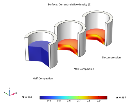
In the Settings window for Surface, click Replace Expression in the upper-right corner of the Expression section. From the menu, choose Component 1 (comp1)>Solid Mechanics>Porous plasticity>solid.lemm1.popl1.rhorel - Current relative density.
|
|
3
|
|
4
|
|
5
|
Click OK.
|
|
1
|
|
2
|
In the Settings window for Surface, click Replace Expression in the upper-right corner of the Expression section. From the menu, choose Component 1 (comp1)>Solid Mechanics>Porous plasticity>solid.lemm1.popl1.rhorel - Current relative density.
|
|
1
|
|
2
|
In the Settings window for Surface, click Replace Expression in the upper-right corner of the Expression section. From the menu, choose Component 1 (comp1)>Solid Mechanics>Porous plasticity>solid.lemm1.popl1.rhorel - Current relative density.
|
|
1
|
|
2
|
|
3
|
|
4
|
|
1
|
|
2
|
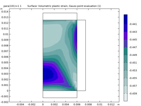
In the tree, select Study 1/Solution 1 (1) (sol1)>Solid Mechanics>Volumetric Plastic Strain (solid).
|
|
3
|
|
4
|
|
1
|
|
2
|
|
3
|
|
4
|
|
5
|
|
6
|
|
1
|
|
2
|
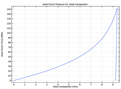
In the Settings window for 1D Plot Group, type Axial Punch Pressure Vs. Axial Compaction in the Label text field.
|
|
3
|
|
4
|
|
5
|
|
6
|
|
1
|
|
2
|
|
4
|
|
5
|
|
6
|
|
7
|
|
8
|
|
1
|
|
2
|
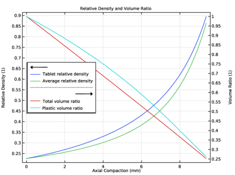
In the Settings window for 1D Plot Group, type Relative Density and Volume Ratio in the Label text field.
|
|
3
|
|
4
|
|
5
|
|
6
|
|
7
|
|
8
|
|
9
|
|
10
|
|
1
|
|
2
|
|
4
|
|
5
|
|
6
|
|
7
|
|
1
|
|
2
|
|
3
|
|
4
|
|
5
|
|
6
|
|
1
|
|
2
|
|
1
|
|
2
|
|
3
|
|
4
|
|
5
|