You are viewing the documentation for an older COMSOL version. The latest version is available here.
PDF

Pressurized Orthotropic Container — Shell Version
Introduction
A container made of rolled steel is subjected to an internal overpressure. As an effect of the manufacturing method of the steel sheet, one of the three material principal directions — the out-of- plane direction — has a higher yield stress than the other two. Hill’s orthotropic plasticity is used to model the differences in yield strength.
This example demonstrates how to perform the analysis of the container using the Shell interface and the Layered Linear Elastic Material.
Model Definition
The metal container has the shape of a cylinder capped by two torispherical heads (also called Klöpper head). The cylinder has an internal radius of Ri = 24 cm, a height of h = 80 cm, and its thickness is t = 2 cm. The torispherical head is made out of three parts: the crown, the knuckle and the flange. The crown has an internal radius of Rc = 43.2 cm, the knuckle has an internal radius of Rk = 5.2 cm, and the straight flange is s = 7 cm in height, see Figure 1.
Figure 1: Schematic description of the container geometry and dimensions.
Because of 2D axial symmetry and reflection symmetry, it is sufficient to model a quarter of the container, see Figure 1. The red lines define the rotation symmetry axis and the reflection symmetry axis.
Material Model
The elastoplastic material is defined by a Young’s modulus, E = 205 GPa and a Poisson’s ratio, ν = 0.28. Hill’s orthotropic plasticity governs the yielding, with the yield stress components given by
There is no hardening, so the material is perfectly plastic. The numbers in the subscripts denote the principal material directions, as indicated in the following section.
Material Orientation
The rolled steel sheet has better mechanical properties in the out-of-plane direction, direction 3. To account for this anisotropy, use a special coordinate system that follows the component shape has to be used, see Figure 2. When using the Shell interface, this coordinate system coincides with the local coordinates of the shell.
Figure 2: Orientation of local material coordinate system. The second principal direction is oriented in the circumferential (out-of-plane) direction, perpendicular to the rz-plane.
Results and Discussion
An approximate analytical solution can be obtained for the cylindrical part of the container. The principal stresses in the center of the container can be estimated from the internal radius Ri, the wall thickness t and internal pressure p:
(1)
Following Hill’s criterion, the yielding occurs when
or replacing by the expressions in Equation 1
The material parameters, F = G = 2.47·1018 1/Pa2 and H = 4.42·1018 1/Pa2, give the analytical onset of yielding in the center of the cylinder at p = 37.8 MPa. Given the curvature of the knuckle, the material in the torispherical head undergoes plastic deformation below this onset pressure.
Figure 3 shows the von Mises stress at 10% yielded volume, which happens when the inner pressure reaches 30.4 MPa. For isotropic steel with yield stress of 381 MPa, the 10% yielded volume is reached when p = 28.4 MPa. Therefore, with orthotropic steel, the pressure needed to reach 10% yielded volume is about 7% higher than when using an isotropic steel sheet. The extent of plastic strains is shown in Figure 4.
Figure 3: Distribution of von Mises stress at 10% yielded volume.
Figure 4: Equivalent plastic strain at 10% yielded volume.
Notes About the COMSOL Implementation
The structure is modeled with the Shell interface and the Layered Linear Elastic Material model. This feature enables to model phenomena that are thickness dependent, such as Plasticity. The user interface is similar to what is available in the Solid Mechanics interface.
Hill orthotropic plasticity is available in COMSOL as a built-in option under the Plasticity node, where either Hill’s coefficients or initial yield stresses can be given. The yield strength values can also be specified in the material node.
Figure 5 visualizes the boundary system and the thickness of the shell. The red arrows denote direction 1, while the blue arrows denote direction 3. The out-of-plane direction is used as direction 2 (not plotted). The normal is oriented to the interior of the container, which enables to directly apply the inner pressure load, see Figure 6.
Figure 5: Thickness of the shell and orientation of the boundary system.
Figure 6: Orientation and amplitude of the applied pressure load.
A stop condition is added to the parametric solver, so that the simulation stops when 10% of the material has exceeded the yield limit. Unless you are performing a failure analysis, it is not necessary to compute the whole plastic history, and the stop condition saves much computation time from being spent in the strongly nonlinear regime.
Application Library path: Nonlinear_Structural_Materials_Module/Plasticity/orthotropic_container_shell
Modeling Instructions
From the File menu, choose New.
New
In the New window, click  Model Wizard.
Model Wizard
1
In the Model Wizard window, click  2D Axisymmetric.
2
In the Select Physics tree, select Structural Mechanics>Shell (shell).
3
Click Add.
4
Click  Study.
5
In the Select Study tree, select General Studies>Stationary.
6
Global Definitions
Parameters 1
1
In the Model Builder window, under Global Definitions click Parameters 1.
2
In the Settings window for Parameters, locate the Parameters section.
3
Click  Load from File.
4
Geometry 1
Crown
1
In the Geometry toolbar, click  More Primitives and choose Circular Arc.
2
In the Settings window for Circular Arc, type Crown in the Label text field.
3
Locate the Center section. In the z text field, type sf-(Rc-hi).
4
Locate the Radius section. In the Radius text field, type Rc.
5
Locate the Angles section. In the Start angle text field, type 90-alpha.
Knuckle
1
In the Geometry toolbar, click  More Primitives and choose Circular Arc.
2
In the Settings window for Circular Arc, type Knuckle in the Label text field.
3
Locate the Center section. In the r text field, type Ri-Rk.
4
In the z text field, type sf.
5
Locate the Radius section. In the Radius text field, type Rk.
6
Locate the Angles section. In the End angle text field, type 90-alpha.
Flange
1
In the Geometry toolbar, click  More Primitives and choose Line Segment.
2
In the Settings window for Line Segment, type Flange in the Label text field.
3
Locate the Starting Point section. From the Specify list, choose Coordinates.
4
In the r text field, type Ri.
5
In the z text field, type sf.
6
Locate the Endpoint section. From the Specify list, choose Coordinates.
7
In the r text field, type Ri.
Cylinder
1
In the Geometry toolbar, click  More Primitives and choose Line Segment.
2
In the Settings window for Line Segment, type Cylinder in the Label text field.
3
Locate the Starting Point section. From the Specify list, choose Coordinates.
4
In the r text field, type Ri.
5
Locate the Endpoint section. From the Specify list, choose Coordinates.
6
In the r text field, type Ri.
7
In the z text field, type -hcyl.
8
Click  Build All Objects.
Definitions
Integration 1 (intop1)
1
In the Definitions toolbar, click  Nonlocal Couplings and choose Integration.
2
In the Settings window for Integration, locate the Source Selection section.
3
From the Geometric entity level list, choose Boundary.
4
From the Selection list, choose All boundaries.
5
Locate the Advanced section. From the Frame list, choose Material  (R, PHI, Z).
Variables 1
1
In the Definitions toolbar, click  Local Variables.
2
In the Settings window for Variables, locate the Variables section.
3
The shell.llem1.xdintopall operator integrates the argument quantity across the thickness.
Set the boundary system to have the first tangent vector oriented upward and the normal oriented to the interior as shown on Figure 5. The latter will make it easier to apply the internal pressure.
Boundary System 1 (sys1)
1
In the Model Builder window, click Boundary System 1 (sys1).
2
In the Settings window for Boundary System, locate the Settings section.
3
Find the Coordinate names subsection. From the Axis list, choose z.
4
Select the Reverse normal direction check box.
Shell (shell)
Layered Linear Elastic Material 1
1
In the Model Builder window, under Component 1 (comp1) right-click Shell (shell) and choose Material Models>Layered Linear Elastic Material.
2
In the Settings window for Layered Linear Elastic Material, locate the Boundary Selection section.
3
From the Selection list, choose All boundaries.
Plasticity 1
1
In the Physics toolbar, click  Attributes and choose Plasticity.
2
In the Settings window for Plasticity, locate the Plasticity Model section.
3
From the σe list, choose Hill orthotropic.
4
Find the Isotropic hardening model subsection. From the list, choose Perfectly plastic.
Symmetry Plane 1
1
In the Physics toolbar, click  Points and choose Symmetry Plane.
2
Face Load 1
1
In the Physics toolbar, click  Boundaries and choose Face Load.
2
In the Settings window for Face Load, locate the Boundary Selection section.
3
From the Selection list, choose All boundaries.
4
Locate the Force section. From the Load type list, choose Pressure.
5
In the p text field, type pressure.
Add Material
1
In the Home toolbar, click  Add Material to open the Add Material window.
2
Go to the Add Material window.
3
In the tree, select Built-in>Steel AISI 4340.
4
Click Add to Component in the window toolbar.
5
In the Home toolbar, click  Add Material to close the Add Material window.
Materials
Steel AISI 4340 (mat1)
1
In the Settings window for Material, locate the Material Contents section.
2
Five elements are set across the thickness to have same discretization as in the solid version of the model.
Since the geometry represents the inner side of the container and the normal is oriented to the interior, the geometry should be the top face of the shell layer.
3
Locate the Orientation and Position section. From the Position list, choose Top side on boundary.
4
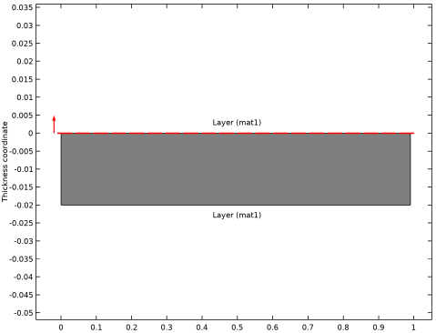
Click Layer Cross-Section Preview in the upper-right corner of the Orientation and Position section.
Mesh 1
Distribution 1
1
In the Model Builder window, under Component 1 (comp1) right-click Mesh 1 and choose Distribution.
2
3
In the Settings window for Distribution, locate the Distribution section.
4
In the Number of elements text field, type 10.
Distribution 2
1
In the Model Builder window, right-click Mesh 1 and choose Distribution.
2
3
In the Settings window for Distribution, locate the Distribution section.
4
In the Number of elements text field, type 25.
Edge 1
1
In the Mesh toolbar, click  Edge.
2
In the Settings window for Edge, locate the Boundary Selection section.
3
From the Selection list, choose All boundaries.
4
Click  Build All.
Study 1
Step 1: Stationary
1
In the Model Builder window, under Study 1 click Step 1: Stationary.
2
In the Settings window for Stationary, click to expand the Study Extensions section.
3
Select the Auxiliary sweep check box.
4
5
6
Introduce a stop condition to stop the solver when a certain amount of material has yielded.
Solution 1 (sol1)
1
In the Study toolbar, click  Show Default Solver.
2
In the Model Builder window, expand the Solution 1 (sol1) node.
3
In the Model Builder window, expand the Study 1>Solver Configurations>Solution 1 (sol1)>Stationary Solver 1 node.
4
Right-click Study 1>Solver Configurations>Solution 1 (sol1)>Stationary Solver 1>Parametric 1 and choose Stop Condition.
5
In the Settings window for Stop Condition, locate the Stop Expressions section.
6
7
Specify that the solution is to be stored both before and after the stop condition is reached.
8
Locate the Output at Stop section. From the Add solution list, choose Steps before and after stop.
9
Clear the Add warning check box.
10
In the Study toolbar, click  Compute.
Results
Surface 1
1
In the Model Builder window, expand the Stress (shell) node, then click Surface 1.
2
In the Settings window for Surface, locate the Expression section.
3
From the Unit list, choose MPa.
Stress (shell)
Surface 1
1
In the Model Builder window, expand the Results>Stress, 3D (shell) node, then click Surface 1.
2
In the Settings window for Surface, locate the Expression section.
3
From the Unit list, choose MPa.
4
In the Stress, 3D (shell) toolbar, click  Plot.
5
In the Home toolbar, click  Add Predefined Plot.
Add Predefined Plot
1
Go to the Add Predefined Plot window.
2
In the tree, select Study 1/Solution 1 (sol1)>Shell>Equivalent Plastic Strain (shell).
3
Click Add Plot in the window toolbar.
4
In the tree, select Study 1/Solution 1 (sol1)>Shell>Stress, Through Thickness (shell).
5
Click Add Plot in the window toolbar.
6
In the tree, select Study 1/Solution 1 (sol1)>Shell>Thickness and Orientation (shell).
7
Click Add Plot in the window toolbar.
8
In the tree, select Study 1/Solution 1 (sol1)>Shell>Applied Loads (shell).
9
Click Add Plot in the window toolbar.
10
In the Home toolbar, click  Add Predefined Plot.
Results
Equivalent Plastic Strain (shell)
1
In the Model Builder window, under Results click Equivalent Plastic Strain (shell).
2
In the Equivalent Plastic Strain (shell) toolbar, click  Plot.
Through Thickness 1
1
In the Model Builder window, expand the Stress, Through Thickness (shell) node, then click Through Thickness 1.
2
In the Settings window for Through Thickness, locate the Selection section.
3
Click  Clear Selection.
4
5
Locate the x-Axis Data section. From the Unit list, choose MPa.
6
In the Stress, Through Thickness (shell) toolbar, click  Plot.
Improve the orientation plot group to show the true thickness of the geometry.
Thickness
1
In the Model Builder window, expand the Thickness and Orientation (shell) node.
2
Right-click Results>Thickness and Orientation (shell)>Thickness and choose Delete.
Thickness and Orientation (shell)
In the Model Builder window, under Results click Thickness and Orientation (shell).
Surface 1
1
In the Thickness and Orientation (shell) toolbar, click  Surface.
2
In the Settings window for Surface, locate the Data section.
3
From the Dataset list, choose Layered Material.
4
From the Solution parameters list, choose From parent.
5
Locate the Expression section. In the Expression text field, type 1.
6
Locate the Coloring and Style section. From the Coloring list, choose Uniform.
7
From the Color list, choose Gray.
Shell Local System
1
In the Model Builder window, click Shell Local System.
2
In the Settings window for Coordinate System Line, locate the Positioning section.
3
In the Number of points text field, type 15.
The onset of plasticity can be investigated by evaluating the volume of the material which has exceeded the yield stress.
Yielded Volume
1
In the Home toolbar, click  Add Plot Group and choose 1D Plot Group.
2
In the Settings window for 1D Plot Group, type Yielded Volume in the Label text field.
3
Locate the Legend section. Clear the Show legends check box.
Global 1
1
In the Yielded Volume toolbar, click  Global.
2
In the Settings window for Global, locate the y-Axis Data section.
3
4
In the Yielded Volume toolbar, click  Plot.