PDF

Wrinkling of Cylindrical Membranes with Varying Thickness
Introduction
The numerical treatment of wrinkling in membranes can be handled by two approaches, see Ref. 1. In the first approach, out-of-plane geometric nonlinearities are treated as constitutive nonlinearities through a modification of the strain energy density, which is called the relaxed strain energy approach. In contrast, the second method involves direct modifications of the deformation gradient instead of the constitutive relation. The second approach is more general and applicable to anisotropic membranes, and this method is implemented in COMSOL Multiphysics.
In this example, wrinkling is studied in a cylindrical membrane of nonuniform thickness that is being stretched axially and filled with water internally. The membrane material is described with an incompressible Mooney–Rivlin model. Depending on the level of axial stretch and internal pressure, certain portions of the membrane undergo wrinkling. The results of the two approaches of handling wrinkling are compared with each other as well as with the results from the example presented in Ref. 1. In the case of the relaxed strain energy approach, the total strain energy for a Mooney–Rivlin material, which is a combination of the full and the relaxed strain energy, is taken from Ref. 1.
Model Definition
The model example is taken from Ref. 1. A cylindrical membrane of radius 10 mm and initial height of 80 mm is first stretched axially and subsequently filled with water. The membrane is modeled with an incompressible two-parameter Mooney–Rivlin hyperelastic material. The material properties are given in Table 1.
C1
C2
The membrane thickness varies along the height as th = thm(2(1 − M)(Z/Hi) + M), where Hi is initial the height, thm is the mean thickness of 0.1 mm, and M is a parameter controlling the variation in thickness, here taken to be 0.5.
Results and Discussions
Figure 1 and Figure 2 show the wrinkled regions in the stretched and inflated cylinder by both approaches at different levels of water column height. The results match with each other approximately; the slight variation in the wrinkled region with the relaxed strain-energy approach comes from the transition zone approximation of the step function.
After stretching, the central portion of the membrane is wrinkled. As the water level increases, the extent of the wrinkling region reduces and finally disappears at around zw= 70 mm. The results are in agreement with those published in Ref. 1.
The first and second principal stresses in the inflated cylinder are shown in Figure 3 and Figure 4, respectively. The stresses from the modified deformation gradient approach matches with the relaxed strain energy approach (see the results from the model). Note that the second principal stress is nonnegative in the whole membrane.
Figure 5 and Figure 6 show the variations in the principal stresses along the height of cylinder after the prestretch. The results from both approaches agree with each other; moreover, the second principal stress is nonnegative in the wrinkled region. Similarly, Figure 7 shows the variation in the third principal strain after prestretch, and both approaches give the same results.
Figure 1: Wrinkled region in the inflated cylinder at different water heights computed with the modified deformation gradient approach.
Figure 2: Wrinkled region in the inflated cylinder at different water heights computed with the relaxed strain energy approach.
Figure 3: First principal stress in the inflated cylinder computed with the modified deformation gradient approach.
Figure 4: Second principal stress in the inflated cylinder with the modified deformation gradient approach.
Figure 5: First principal stress in the cylinder after prestretch.
Figure 6: Second principal stress in the cylinder after prestretch.
Figure 7: Third principal strain in the cylinder after prestretch.
Notes About the COMSOL Implementation
A wrinkling model based on the modified deformation gradient is incorporated within the membrane theory using the Wrinkling feature, which solves a set of nonlinear equations with the Newton–Raphson method.
The strain energy density based on the relaxed strain energy approach is taken from Ref. 1 and implemented through the User Defined option under the Hyperelastic Material node. A weak contribution is added to enforce material incompressibility. Furthermore, wrinkling is identified to occur in the limit when the second principal stress turns negative (uniaxial stress conditions). Because the material is isotropic and incompressible, the wrinkling condition can thus be formulated in terms of the in-plane principal stretches as
(1)
Reference
1. A. Patil, “Inflation and instabilities of hyperelastic membranes,” PhD Thesis, KTH, 2016.
Application Library path: Nonlinear_Structural_Materials_Module/Hyperelasticity/membrane_varying_thickness
Modeling Instructions
From the File menu, choose New.
New
In the New window, click  Model Wizard.
Model Wizard
1
In the Model Wizard window, click  2D Axisymmetric.
2
In the Select Physics tree, select Structural Mechanics>Membrane (mbrn).
3
Click Add.
4
Click  Study.
5
In the Select Study tree, select General Studies>Stationary.
6
Global Definitions
Model Parameters
1
In the Model Builder window, under Global Definitions click Parameters 1.
2
In the Settings window for Parameters, type Model Parameters in the Label text field.
3
Locate the Parameters section. Click  Load from File.
4
Definitions
Step 1 (step1)
1
In the Home toolbar, click  Functions and choose Local>Step.
2
In the Settings window for Step, click to expand the Smoothing section.
3
Locate the Parameters section. In the Location text field, type 1.
4
Locate the Smoothing section. In the Size of transition zone text field, type 0.015.
Variables 1
1
In the Model Builder window, right-click Definitions and choose Variables.
2
In the Settings window for Variables, locate the Variables section.
3
Click  Load from File.
4
Geometry 1
Line Segment 1 (ls1)
1
In the Geometry toolbar, click  More Primitives and choose Line Segment.
2
In the Settings window for Line Segment, locate the Starting Point section.
3
From the Specify list, choose Coordinates.
4
In the r text field, type Ri.
5
Locate the Endpoint section. From the Specify list, choose Coordinates.
6
In the r text field, type Ri.
7
In the z text field, type Hi.
8
Click  Build Selected.
Membrane (mbrn)
Thickness and Offset 1
1
In the Model Builder window, under Component 1 (comp1)>Membrane (mbrn) click Thickness and Offset 1.
2
In the Settings window for Thickness and Offset, locate the Thickness and Offset section.
3
In the d0 text field, type th.
To model wrinkling using the built-in modified deformation gradient approach, add a Mooney–Rivlin hyperelastic material with a Wrinkling subfeature.
Hyperelastic Material (Modified Deformation Gradient Approach)
1
In the Physics toolbar, click  Boundaries and choose Hyperelastic Material.
2
3
In the Settings window for Hyperelastic Material, type Hyperelastic Material (Modified Deformation Gradient Approach) in the Label text field.
4
Locate the Hyperelastic Material section. From the Material model list, choose Mooney-Rivlin, two parameters.
5
From the Compressibility list, choose Incompressible.
6
From the C10 list, choose User defined. In the associated text field, type C1.
7
From the C01 list, choose User defined. In the associated text field, type C2.
Wrinkling 1
1
In the Physics toolbar, click  Attributes and choose Wrinkling.
2
In the Settings window for Wrinkling, locate the Wrinkling section.
3
From the Termination criterion for local method list, choose Step size or residual.
To model wrinkling using the relaxed strain energy approach, add a user-defined hyperelastic material.
Hyperelastic Material (Relaxed Strain Energy Approach)
1
In the Physics toolbar, click  Boundaries and choose Hyperelastic Material.
The energy expression considers incompressibility implicitly, hence we do not need to use the built-in mixed formulation coming with Nearly incompressible or Incompressible models. Therefore, choose the Compressible option.
2
In the Settings window for Hyperelastic Material, locate the Boundary Selection section.
3
From the Selection list, choose All boundaries.
4
In the Label text field, type Hyperelastic Material (Relaxed Strain Energy Approach).
5
Locate the Hyperelastic Material section. From the Material model list, choose User defined.
6
In the Ws text field, type WT.
7
Click the  Show More Options button in the Model Builder toolbar.
8
In the Show More Options dialog box, click  Select All.
9
Add a weak equation to determine the normal strain for the relaxed strain energy approach.
Weak Contribution 1
1
In the Physics toolbar, click  Boundaries and choose Weak Contribution.
2
3
In the Settings window for Weak Contribution, locate the Weak Contribution section.
4
In the Weak expression text field, type (-1+mbrn.Jel)*test(mbrn.unn).
Prescribed Displacement 1
1
In the Physics toolbar, click  Points and choose Prescribed Displacement.
2
3
In the Settings window for Prescribed Displacement, locate the Prescribed Displacement section.
4
Select the Prescribed in r direction check box.
5
Select the Prescribed in z direction check box.
Prescribed Displacement (Prestretch)
1
In the Physics toolbar, click  Points and choose Prescribed Displacement.
2
In the Settings window for Prescribed Displacement, type Prescribed Displacement (Prestretch) in the Label text field.
3
4
Locate the Prescribed Displacement section. Select the Prescribed in r direction check box.
5
Select the Prescribed in z direction check box.
6
In the u0z text field, type w_appl.
Face Load (Fluid Pressure)
1
In the Physics toolbar, click  Boundaries and choose Face Load.
2
3
In the Settings window for Face Load, locate the Force section.
4
From the Load type list, choose Pressure.
5
In the p text field, type P.
6
In the Label text field, type Face Load (Fluid Pressure).
Mesh 1
1
In the Model Builder window, under Component 1 (comp1) click Mesh 1.
2
In the Settings window for Mesh, locate the Physics-Controlled Mesh section.
3
From the Element size list, choose Extra fine.
4
Click  Build All.
Set up two study steps: one for prestretching, and another for inflation. Use the prestretch solution as initial values for the inflation step.
Study (Modified Deformation Gradient Approach)
1
In the Model Builder window, click Study 1.
2
In the Settings window for Study, type Study (Modified Deformation Gradient Approach) in the Label text field.
3
Locate the Study Settings section. Clear the Generate default plots check box.
Prestretch
1
In the Model Builder window, under Study (Modified Deformation Gradient Approach) click Step 1: Stationary.
2
In the Settings window for Stationary, type Prestretch in the Label text field.
3
Locate the Physics and Variables Selection section. Select the Modify model configuration for study step check box.
4
In the tree, select Component 1 (comp1)>Membrane (mbrn), Controls spatial frame>Hyperelastic Material (Relaxed Strain Energy Approach) and Component 1 (comp1)>Membrane (mbrn), Controls spatial frame>Weak Contribution 1.
5
6
In the tree, select Component 1 (comp1)>Membrane (mbrn), Controls spatial frame>Face Load (Fluid Pressure).
7
Inflation
1
In the Study toolbar, click  Study Steps and choose Stationary>Stationary.
2
In the Settings window for Stationary, type Inflation in the Label text field.
3
Click to expand the Values of Dependent Variables section. Locate the Physics and Variables Selection section. Select the Modify model configuration for study step check box.
4
In the tree, select Component 1 (comp1)>Membrane (mbrn), Controls spatial frame>Hyperelastic Material (Relaxed Strain Energy Approach) and Component 1 (comp1)>Membrane (mbrn), Controls spatial frame>Weak Contribution 1.
5
6
Locate the Values of Dependent Variables section. Find the Initial values of variables solved for subsection. From the Settings list, choose User controlled.
7
Click to expand the Study Extensions section. Select the Auxiliary sweep check box.
8
9
10
In the Study toolbar, click  Compute.
Add Study
1
In the Study toolbar, click  Add Study to open the Add Study window.
2
Go to the Add Study window.
3
Find the Studies subsection. In the Select Study tree, select General Studies>Stationary.
4
Click Add Study in the window toolbar.
5
In the Study toolbar, click  Add Study to close the Add Study window.
Study (Relaxed Strain Energy Approach)
1
In the Model Builder window, click Study 2.
2
In the Settings window for Study, type Study (Relaxed Strain Energy Approach) in the Label text field.
3
Locate the Study Settings section. Clear the Generate default plots check box.
Prestretch
1
In the Model Builder window, under Study (Relaxed Strain Energy Approach) click Step 1: Stationary.
2
In the Settings window for Stationary, type Prestretch in the Label text field.
3
Locate the Physics and Variables Selection section. Select the Modify model configuration for study step check box.
4
In the tree, select Component 1 (comp1)>Membrane (mbrn), Controls spatial frame>Face Load (Fluid Pressure).
5
Inflation
1
In the Study toolbar, click  Study Steps and choose Stationary>Stationary.
2
In the Settings window for Stationary, type Inflation in the Label text field.
3
Locate the Values of Dependent Variables section. Find the Initial values of variables solved for subsection. From the Settings list, choose User controlled.
4
From the Method list, choose Solution.
5
From the Study list, choose Study (Relaxed Strain Energy Approach), Prestretch.
6
Locate the Study Extensions section. Select the Auxiliary sweep check box.
7
8
9
In the Study toolbar, click  Compute.
Add two predefined plots, one 2D and one 3D representation. Edit the first to show the wrinkled region in the membrane.
10
In the Home toolbar, click  Add Predefined Plot.
Add Predefined Plot
1
Go to the Add Predefined Plot window.
2
In the tree, select Study (Modified Deformation Gradient Approach)/Solution 1 (sol1)>Membrane>Stress (mbrn).
3
Click Add Plot in the window toolbar.
4
In the tree, select Study (Modified Deformation Gradient Approach)/Solution 1 (sol1)>Membrane>Stress, 3D (mbrn).
5
Click Add Plot in the window toolbar.
6
In the Home toolbar, click  Add Predefined Plot.
Results
Wrinkled Region
1
In the Model Builder window, under Results click Stress (mbrn).
2
In the Settings window for 2D Plot Group, type Wrinkled Region in the Label text field.
3
Click to expand the Plot Array section. Select the Enable check box.
4
In the Relative padding text field, type 25.
Line 1
1
In the Model Builder window, expand the Wrinkled Region node, then click Line 1.
2
In the Settings window for Line, locate the Data section.
3
From the Dataset list, choose Study (Modified Deformation Gradient Approach)/Solution 1 (sol1).
4
From the Parameter value (z_w (mm)) list, choose 0.
5
Locate the Expression section. In the Expression text field, type mbrn.iswrinkled.
6
Locate the Coloring and Style section.
7
Select the Radius scale factor check box. In the associated text field, type 3e-3.
Line 2
1
Right-click Results>Wrinkled Region>Line 1 and choose Duplicate.
2
In the Settings window for Line, locate the Data section.
3
From the Parameter value (z_w (mm)) list, choose 20.
4
Click to expand the Title section. From the Title type list, choose None.
5
Click to expand the Inherit Style section. From the Plot list, choose Line 1.
Line 3
1
Right-click Line 2 and choose Duplicate.
2
In the Settings window for Line, locate the Data section.
3
From the Parameter value (z_w (mm)) list, choose 40.
Line 4
1
Right-click Line 3 and choose Duplicate.
2
In the Settings window for Line, locate the Data section.
3
From the Parameter value (z_w (mm)) list, choose 80.
Wrinkled Region
In the Model Builder window, click Wrinkled Region.
Table Annotation 1
1
In the Wrinkled Region toolbar, click  More Plots and choose Table Annotation.
2
In the Settings window for Table Annotation, click to expand the Plot Array section.
3
Locate the Data section. From the Source list, choose Local table.
4
5
Select the LaTeX markup check box.
6
Locate the Coloring and Style section. Clear the Show point check box.
Wrinkled Region
1
In the Model Builder window, click Wrinkled Region.
2
In the Settings window for 2D Plot Group, click to expand the Title section.
3
From the Title type list, choose Custom.
4
Find the Solution subsection. Clear the Solution check box.
5
Click the  Zoom Extents button in the Graphics toolbar.
6
In the Wrinkled Region toolbar, click  Plot.
Edit the second predefined plot to show the first principal stress in 3D.
First Principal Stress
1
In the Model Builder window, under Results click Stress, 3D (mbrn).
2
In the Settings window for 3D Plot Group, type First Principal Stress in the Label text field.
3
Locate the Data section. From the Dataset list, choose Revolution 2D.
4
Locate the Color Legend section. Select the Show maximum and minimum values check box.
Surface 1
1
In the Model Builder window, expand the First Principal Stress node, then click Surface 1.
2
In the Settings window for Surface, locate the Data section.
3
From the Dataset list, choose From parent.
4
Locate the Expression section. In the Expression text field, type mbrn.sp1.
5
From the Unit list, choose MPa.
6
In the First Principal Stress toolbar, click  Plot.
Duplicate the plot group to also show the second principal stress.
Second Principal Stress
1
In the Model Builder window, right-click First Principal Stress and choose Duplicate.
2
In the Settings window for 3D Plot Group, type Second Principal Stress in the Label text field.
Surface 1
1
In the Model Builder window, expand the Second Principal Stress node, then click Surface 1.
2
In the Settings window for Surface, locate the Expression section.
3
In the Expression text field, type mbrn.sp2.
4
In the Second Principal Stress toolbar, click  Plot.
First Principal Stress, Second Principal Stress, Wrinkled Region
1
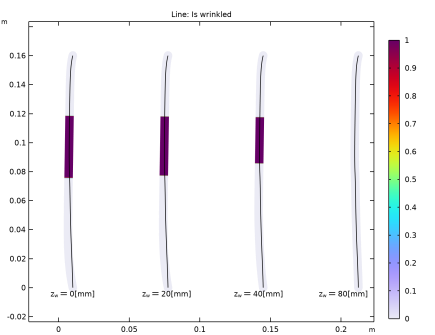
In the Model Builder window, under Results, Ctrl-click to select Wrinkled Region, First Principal Stress, and Second Principal Stress.
2
Modified Deformation Gradient Approach
In the Settings window for Group, type Modified Deformation Gradient Approach in the Label text field.
Relaxed Strain Energy Approach
1
Right-click Modified Deformation Gradient Approach and choose Duplicate.
2
In the Settings window for Group, type Relaxed Strain Energy Approach in the Label text field.
Wrinkled Region 1
1
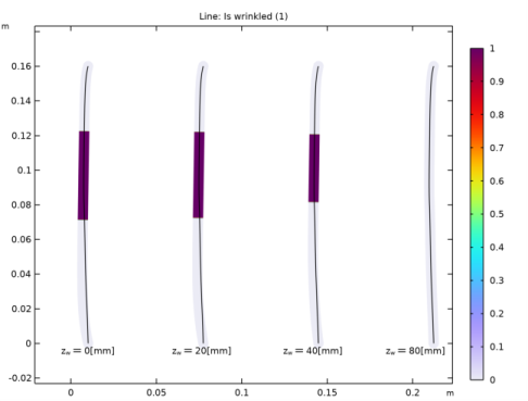
In the Model Builder window, expand the Relaxed Strain Energy Approach node, then click Wrinkled Region 1.
2
In the Settings window for 2D Plot Group, locate the Data section.
3
From the Dataset list, choose Study (Relaxed Strain Energy Approach)/Solution 3 (sol3).
Line 1
1
In the Model Builder window, expand the Wrinkled Region 1 node, then click Line 1.
2
In the Settings window for Line, locate the Data section.
3
From the Dataset list, choose Study (Relaxed Strain Energy Approach)/Solution 3 (sol3).
4
Locate the Expression section. In the Expression text field, type iswrinkled.
Line 2
1
In the Model Builder window, click Line 2.
2
In the Settings window for Line, locate the Data section.
3
From the Dataset list, choose Study (Relaxed Strain Energy Approach)/Solution 3 (sol3).
4
Locate the Expression section. In the Expression text field, type iswrinkled.
Line 3
1
In the Model Builder window, click Line 3.
2
In the Settings window for Line, locate the Data section.
3
From the Dataset list, choose Study (Relaxed Strain Energy Approach)/Solution 3 (sol3).
4
Locate the Expression section. In the Expression text field, type iswrinkled.
Line 4
1
In the Model Builder window, click Line 4.
2
In the Settings window for Line, locate the Data section.
3
From the Dataset list, choose Study (Relaxed Strain Energy Approach)/Solution 3 (sol3).
4
Locate the Expression section. In the Expression text field, type iswrinkled.
5
In the Wrinkled Region 1 toolbar, click  Plot.
Revolution 2D 1
1
In the Model Builder window, expand the Results>Datasets node.
2
Right-click Revolution 2D and choose Duplicate.
3
In the Settings window for Revolution 2D, locate the Data section.
4
From the Dataset list, choose Study (Relaxed Strain Energy Approach)/Solution 3 (sol3).
First Principal Stress 1
1
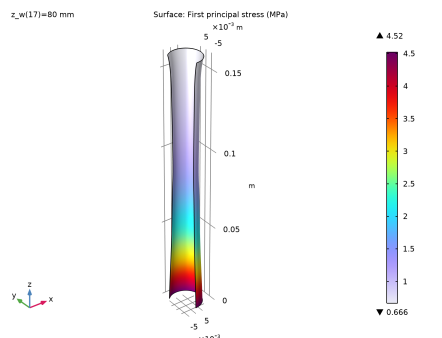
In the Model Builder window, under Results>Relaxed Strain Energy Approach click First Principal Stress 1.
2
In the Settings window for 3D Plot Group, locate the Data section.
3
From the Dataset list, choose Revolution 2D 1.
4
In the First Principal Stress 1 toolbar, click  Plot.
Second Principal Stress 1
1
In the Model Builder window, click Second Principal Stress 1.
2
In the Settings window for 3D Plot Group, locate the Data section.
3
From the Dataset list, choose Revolution 2D 1.
4
In the Second Principal Stress 1 toolbar, click  Plot.
Third Principal Strain after Prestretch
1
In the Home toolbar, click  Add Plot Group and choose 1D Plot Group.
2
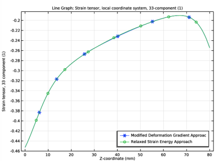
In the Settings window for 1D Plot Group, type Third Principal Strain after Prestretch in the Label text field.
3
Locate the Data section. From the Dataset list, choose Study (Modified Deformation Gradient Approach)/Solution Store 1 (sol2).
4
Locate the Plot Settings section.
5
Select the y-axis label check box. In the associated text field, type Strain tensor, 33 component (1).
6
Locate the Legend section. From the Position list, choose Lower right.
Line Graph 1
1
Right-click Third Principal Strain after Prestretch and choose Line Graph.
2
3
In the Settings window for Line Graph, locate the y-Axis Data section.
4
In the Expression text field, type mbrn.el33.
5
Locate the x-Axis Data section. From the Parameter list, choose Expression.
6
In the Expression text field, type Z.
7
From the Unit list, choose mm.
8
Click to expand the Coloring and Style section. Find the Line markers subsection. From the Marker list, choose Cycle.
9
From the Positioning list, choose Interpolated.
10
In the Number text field, type 6.
11
Click to expand the Legends section. Select the Show legends check box.
12
From the Legends list, choose Manual.
13
Line Graph 2
1
Right-click Line Graph 1 and choose Duplicate.
2
In the Settings window for Line Graph, locate the Data section.
3
From the Dataset list, choose Study (Relaxed Strain Energy Approach)/Solution Store 2 (sol4).
4
Click to expand the Title section. From the Title type list, choose None.
5
Locate the Coloring and Style section. Find the Line markers subsection. In the Number text field, type 8.
6
Locate the Legends section. In the table, enter the following settings:
Third Principal Strain after Prestretch
1
In the Model Builder window, click Third Principal Strain after Prestretch.
2
In the Third Principal Strain after Prestretch toolbar, click  Plot.
First Principal Stress after Prestretch
1
Right-click Third Principal Strain after Prestretch and choose Duplicate.
2
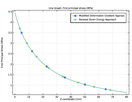
In the Settings window for 1D Plot Group, type First Principal Stress after Prestretch in the Label text field.
3
Locate the Plot Settings section. In the y-axis label text field, type First Principal Stress (MPa).
4
Locate the Legend section. From the Position list, choose Upper right.
Line Graph 1
1
In the Model Builder window, expand the First Principal Stress after Prestretch node, then click Line Graph 1.
2
In the Settings window for Line Graph, locate the y-Axis Data section.
3
In the Expression text field, type mbrn.sp1.
4
From the Unit list, choose MPa.
Line Graph 2
1
In the Model Builder window, click Line Graph 2.
2
In the Settings window for Line Graph, locate the y-Axis Data section.
3
In the Expression text field, type mbrn.sp1.
4
From the Unit list, choose MPa.
First Principal Stress after Prestretch
1
In the Model Builder window, click First Principal Stress after Prestretch.
2
In the First Principal Stress after Prestretch toolbar, click  Plot.
Second Principal Stress after Prestretch
1
Right-click First Principal Stress after Prestretch and choose Duplicate.
2
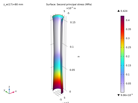
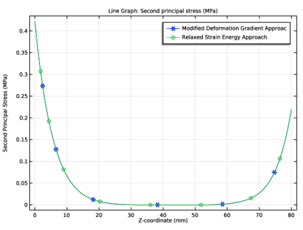
In the Settings window for 1D Plot Group, type Second Principal Stress after Prestretch in the Label text field.
3
Locate the Plot Settings section. In the y-axis label text field, type Second Principal Stress (MPa).
Line Graph 1
1
In the Model Builder window, expand the Second Principal Stress after Prestretch node, then click Line Graph 1.
2
In the Settings window for Line Graph, locate the y-Axis Data section.
3
In the Expression text field, type mbrn.sp2.
Line Graph 2
1
In the Model Builder window, click Line Graph 2.
2
In the Settings window for Line Graph, locate the y-Axis Data section.
3
In the Expression text field, type mbrn.sp2.
4
In the Second Principal Stress after Prestretch toolbar, click  Plot.