Inflation of a Square Hyperelastic Airbag

The numerical treatment of thin structures with a membrane model is much simpler than with a shell model due to the assumption of zero bending stiffness. However, for some load cases this assumption is disadvantageous. For instance, the zero bending stiffness triggers wrinkling when a membrane is subjected to compressive stresses, which result in an equilibrium instability. This limitation can be overcome by the incorporation of a wrinkling model based on the tension field theory.

In this example, a square airbag made of a neo-Hookean hyperelastic material is inflated using pressurized air. The results are compared with the example presented in Ref. 1.

The example is similar to the model Inflation of a Square Airbag in the Structural Mechanics Module Application Library, where a linear elastic material model is used.

Model Definition

A square airbag, 1 mm in thickness and 1.2 m in diagonal length, is inflated using pressurized air. The membrane is modeled as a compressible neo-Hookean hyperelastic material. The material properties given in Table 1 are taken from Ref. 1.

Table 1: Material properties.
Property	Variable	Value
Young’s modulus	E	588 MPa
Poisson’s ratio	ν	0.4

Only a quarter of the airbag is analyzed due to the intrinsic symmetry of the model.

Results and Discussions

Figure 1 shows the wrinkled regions in the inflated airbag. Apart from the central region, wrinkles develop everywhere.

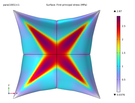
The transverse displacement of the inflated airbag is shown in Figure 2. The distribution of the first and second principal stress at the end of the inflation process is shown in Figure 3 and Figure 4, respectively. The minimum value of the second principal stress is almost zero. Both figures show tensile principal stresses after inflation.

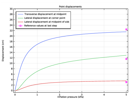
Figure 5 shows the displacement of three different material points as a function of the inflation pressure. These displacements are compared with the results given in Ref. 1. At the final pressure, the values match the reference values well. Figure 6 shows the variation in the first principal (tensile) stress in the midpoint of the airbag with the inflation pressure.

Figure 1: Wrinkled region in the inflated airbag.

Figure 2: Transverse displacement after inflation.

Figure 3: First principal stress after inflation.

Figure 4: Second principal stress after inflation.

Figure 5: Displacements at different material points during inflation.

Figure 6: First principal stress in the airbag center during inflation.

Notes About the COMSOL Implementation

A wrinkling model based on the modified deformation gradient is incorporated within the membrane theory using the feature, which solves a set of nonlinear equations with the Newton–Raphson method.

Since the unstressed membrane does not have any stiffness in the normal direction, a very small spring support is added to stabilize the model. To further improve the numerical stability, a load support is provided in the form of an edge load that decreases parametrically as the model becomes stable when the membrane is under tension.

Constant strain triangle (CST) elements are numerically stable for wrinkling problems. CST elements give constant strains, which in turn give constant stresses for homogeneous material properties, ensuring that the whole element is either wrinkled, slack, or taut. This type of elements are used for the analysis.

Reference

1. A. Diaby, A.L. Van, and C. Wielgosz, “Wrinkling and buckling of prestressed membranes,” Finite Elem. Anal. Des., vol. 42, no. 11, pp. 992–1001, 2006.

Nonlinear_Structural_Materials_Module/Hyperelasticity/membrane_airbag_inflation_hyperelastic

Modeling Instructions

From the menu, choose .

New

In the window, click

Model Wizard

In the window, click

In the tree, select .

Click .

Click

In the tree, select .

Click

Global Definitions

Model Parameters

In the window, under click .

In the window for , type Model Parameters in the text field.

Locate the section. Click

Browse to the model’s Application Libraries folder and double-click the file membrane_airbag_inflation_hyperelastic_parameters.txt.

Definitions

Interpolation 1 (int1)

In the toolbar, click

and choose .

In the window for , locate the section.

In the text field, type F.

In the table, enter the following settings:


t	f(t)
0	100
1	1

Locate the section. In the table, enter the following settings:


Function	Unit
F	N/m

In the table, enter the following settings:


Argument	Unit
t	1

Variables 1

In the window, right-click and choose .

In the window for , locate the section.

In the table, enter the following settings:


Name	Expression	Unit	Description
wmax_ref	22.45[cm]	m	Transverse displacement at midpoint, reference
u1max_ref	3.07[cm]	m	Lateral displacement at corner point, reference
u2max_ref	11.58[cm]	m	Lateral displacement at midpoint of side edge, reference

Due to symmetry, only a quarter of the geometry is constructed.

Geometry 1

Work Plane 1 (wp1)

In the window, expand the node.

Right-click and choose .

Work Plane 1 (wp1)>Square 1 (sq1)

In the toolbar, click

In the window for , locate the section.

In the text field, type L/2.

Locate the section. In the text field, type L/2.

In the toolbar, click

Materials

Material 1 (mat1)

In the window, under right-click and choose .

When modeling wrinkling, constant strain triangular (CST) elements are a good choice due to their numerical stability. Use a triangular mesh and change the default discretization to .

Membrane (mbrn)

In the window for , click to expand the section.

From the list, choose .

Hyperelastic Material 1

Right-click and choose .

In the window for , locate the section.

From the list, choose .

Locate the section. From the list, choose .

Wrinkling 1

In the toolbar, click

and choose .

Wrinkling 1

In the window, expand the node, then click .

In the window for , locate the section.

From the list, choose .

Thickness and Offset 1

In the window, under click .

In the window for , locate the section.

In the d0 text field, type th.

Symmetry 1

In the toolbar, click

and choose .

Select Edges 1 and 3 only.

Prescribed Displacement 1

In the toolbar, click

and choose .

Select Edges 2 and 4 only.

In the window for , locate the section.

Select the check box.

Face Load 1

In the toolbar, click

and choose .

Select Boundary 1 only.

In the window for , locate the section.

From the list, choose .

In the p text field, type -Pmax*para.

Add a parametrically decreasing edge load on the outer edges in the lateral direction in form of a spring force in order to increase the numerical stability. Note that the local edge coordinate system is used.

Edge Load 1

In the toolbar, click

and choose .

Select Edges 2 and 4 only.

In the window for , locate the section.

From the list, choose .

Locate the section. Specify the FL vector as


0	xl
-F(para)	yl
0	zl

Add a spring support in the thickness direction in order to improve numerical stability.

Spring Foundation 1

In the toolbar, click

and choose .

In the window for , locate the section.

From the list, choose .

Locate the section. From the list, choose .

In the kA table, enter the following settings:


0	0	0
0	0	0
0	0	1e-3[N/m^3]

Materials

Material 1 (mat1)

In the window, under click .

In the window for , locate the section.

In the table, enter the following settings:


Property	Variable	Value	Unit	Property group
Young’s modulus	E	EE	Pa	Young’s modulus and Poisson’s ratio
Poisson’s ratio	nu	Nu	1	Young’s modulus and Poisson’s ratio
Density	rho	0	kg/m³	Basic