
|
|
|

|
1
|
|
2
|
|
3
|
Click Add.
|
|
4
|
Click
|
|
5
|
|
6
|
Click
|
|
1
|
|
2
|
|
3
|
|
4
|
Click
|
|
5
|
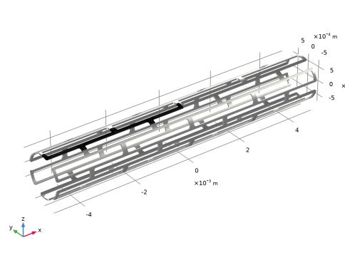
Browse to the model’s Application Libraries folder and double-click the file biomedical_stent.mphbin.
|
|
6
|
Click
|
|
7
|
|
1
|
|
2
|
|
3
|
|
1
|
In the Model Builder window, under Component 1 (comp1) right-click Materials and choose Blank Material.
|
|
2
|
|
4
|
|
1
|
|
2
|
|
3
|
|
4
|
|
5
|
|
6
|
|
1
|
|
2
|
|
1
|
|
2
|
|
3
|
|
5
|
|
1
|
|
2
|
|
3
|
|
4
|
Find the Intervals subsection. In the table, enter the following settings:
|
|
5
|
|
6
|
|
7
|
Click
|
|
1
|
|
1
|
|
3
|
|
4
|
|
5
|
|
6
|
|
7
|
In the Show More Options dialog box, in the tree, select the check box for the node Physics>Equation-Based Contributions.
|
|
8
|
Click OK.
|
|
1
|
|
2
|
|
4
|
|
5
|
|
6
|
Click
|
|
7
|
|
8
|
Click OK.
|
|
9
|
|
10
|
|
11
|
|
12
|
Click
|
|
13
|
|
14
|
Click OK.
|
|
1
|
|
1
|
|
2
|
|
3
|
Click the Custom button.
|
|
4
|
|
5
|
|
6
|
|
7
|
|
8
|
|
1
|
|
2
|
|
3
|
|
4
|
|
1
|
|
2
|
|
3
|
|
5
|
|
6
|
|
1
|
|
2
|
|
3
|
|
5
|
|
6
|
|
1
|
|
2
|
|
1
|
|
2
|
|
1
|
|
2
|
|
3
|
|
4
|
Click
|
|
1
|
|
2
|
|
3
|
In the Model Builder window, expand the Study 1>Solver Configurations>Solution 1 (sol1)>Dependent Variables 1 node, then click Pressure (comp1.ODE1).
|
|
4
|
|
5
|
|
6
|
|
7
|
In the Model Builder window, expand the Study 1>Solver Configurations>Solution 1 (sol1)>Stationary Solver 1 node.
|
|
8
|
Right-click Study 1>Solver Configurations>Solution 1 (sol1)>Stationary Solver 1>Parametric 1 and choose Stop Condition.
|
|
9
|
|
10
|
Click
|
|
12
|
|
13
|
|
14
|
|
1
|
|
2
|
|
3
|
|
4
|
|
1
|
|
2
|
|
1
|
|
2
|
|
3
|
|
4
|
|
1
|
|
2
|
|
3
|
|
4
|
|
5
|
|
1
|
|
2
|
|
3
|
|
4
|
|
1
|
|
2
|
|
3
|
|
1
|
|
2
|
|
3
|
|
1
|
|
2
|
|
1
|
|
2
|
|
3
|
|
1
|
|
2
|
|
3
|
|
4
|
|
1
|
|
2
|
|
1
|
|
2
|
|
3
|
|
1
|
|
2
|
|
3
|
|
1
|
|
2
|
|
1
|
|
2
|
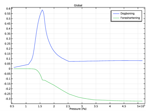
In the Settings window for 1D Plot Group, type Dogboning and Foreshortening in the Label text field.
|
|
3
|
|
1
|
|
2
|
In the Settings window for Global, click Replace Expression in the upper-right corner of the y-Axis Data section. From the menu, choose Component 1 (comp1)>Definitions>Variables>dogboning - Dogboning.
|
|
3
|
Click Add Expression in the upper-right corner of the y-Axis Data section. From the menu, choose Component 1 (comp1)>Definitions>Variables>foreshortening - Foreshortening.
|
|
4
|
Click Replace Expression in the upper-right corner of the x-Axis Data section. From the menu, choose Component 1 (comp1)>Solid Mechanics>p - Pressure - Pa.
|
|
5
|
|
6
|
|
7
|
|
8
|
|
1
|
|
2
|
|
3
|
|
4
|
|
1
|
|
2
|
|
4
|
|
1
|
|
2
|
|
3
|
|
1
|
|
2
|
|
3
|
|
1
|
|
2
|
|
3
|
|
4
|