|
|
|

|
•
|
Inlet (z = 0)
|
|
•
|
|
•
|
|
•
|
Inlet (z = 0)
|
|
•
|
|
•
|
|
•
|
Inlet (z = 0)
|
|
•
|
|
•
|
Frequency factor, A = 16.96E12 1/h
|
|
•
|
|
•
|
Thermal conductivity of the reaction mixture, ke = 0.559 W/(m·K)
|
|
•
|
|
•
|
Inlet temperature, T0 = 312 K
|
|
•
|
Inlet temperature of the coolant, Ta0 = 277 K
|
|
•
|
|
•
|
|
•
|
Mass flow rate of coolant, mc = 0.1 kg/s
|
|
•
|
|
•
|
|
•
|
|
•
|
Heat capacity at inlet, Cp0 = (146.54*cA0_po+75.36*cB0+81.095*cMe0)/rho0 J/(kg·K) (here, the numerical factors are the molar specific heat values in the unit J/(mol·K))
|
|
•
|
Heat capacity per mass of coolant, Cpc = 4180 J/(kg·K)
|
|
•
|
|
•
|
Reactor radius, Ra = 0.1 m
|
|
•
|
Reactor length, L = 1 m
|
|
•
|
|
•
|
|
•
|
|
1
|
|
2
|
|
3
|
Click Add.
|
|
4
|
|
5
|
|
6
|
Click Add.
|
|
7
|
In the Select Physics tree, select Mathematics>PDE Interfaces>Lower Dimensions>Coefficient Form Boundary PDE (cb).
|
|
8
|
Click Add.
|
|
9
|
In the Dependent variables table, enter the following settings:
|
|
10
|
|
11
|
|
12
|
Click
|
|
13
|
|
14
|
Click OK.
|
|
15
|
|
16
|
click
|
|
17
|
|
18
|
Click
|
|
1
|
|
2
|
|
3
|
|
4
|
|
5
|
|
1
|
|
2
|
|
3
|
|
4
|
Browse to the model’s Application Libraries folder and double-click the file tubular_reactor_parameters.txt.
|
|
1
|
|
2
|
|
3
|
|
4
|
Browse to the model’s Application Libraries folder and double-click the file tubular_reactor_variables.txt.
|
|
1
|
In the Model Builder window, under Component 1 (comp1)>Transport of Diluted Species (tds) click Transport Properties 1.
|
|
2
|
|
3
|
Specify the u vector as
|
|
4
|
|
1
|
|
2
|
|
3
|
|
1
|
|
3
|
|
4
|
|
1
|
|
3
|
|
4
|
|
5
|
|
1
|
|
1
|
|
2
|
|
3
|
Specify the u vector as
|
|
4
|
Locate the Heat Conduction, Fluid section. From the k list, choose User defined. In the associated text field, type ke.
|
|
5
|
|
6
|
|
7
|
|
8
|
|
1
|
|
2
|
|
3
|
|
1
|
|
3
|
|
4
|
|
1
|
|
3
|
|
4
|
|
1
|
|
3
|
|
4
|
|
1
|
|
1
|
|
2
|
|
3
|
|
4
|
|
1
|
In the Model Builder window, under Component 1 (comp1)>Coefficient Form Boundary PDE (cb) click Coefficient Form PDE 1.
|
|
2
|
|
3
|
|
4
|
|
5
|
|
1
|
|
3
|
In the Settings window for Dirichlet Boundary Condition, locate the Dirichlet Boundary Condition section.
|
|
4
|
|
1
|
|
3
|
|
4
|
|
5
|
|
6
|
|
7
|
|
8
|
|
1
|
|
3
|
|
4
|
|
5
|
|
6
|
|
7
|
|
8
|
|
9
|
|
1
|
|
1
|
|
2
|
|
3
|
|
4
|
|
1
|
|
2
|
|
3
|
|
4
|
|
5
|
|
1
|
|
2
|
|
3
|
|
4
|
|
5
|
|
6
|
|
7
|
|
8
|
|
1
|
|
2
|
In the Settings window for Surface, click Replace Expression in the upper-right corner of the Expression section. From the menu, choose Component 1 (comp1)>Heat Transfer in Fluids>Temperature>T - Temperature - K.
|
|
3
|
|
4
|
|
1
|
|
2
|
|
3
|
|
1
|
|
2
|
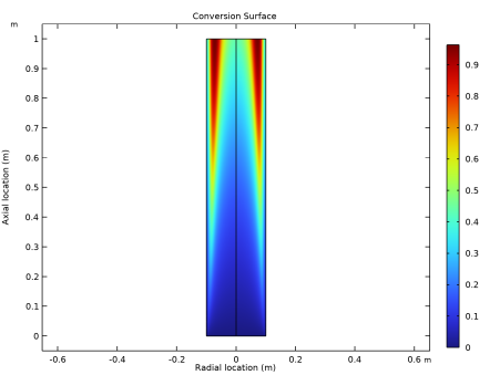
In the Settings window for Surface, click Replace Expression in the upper-right corner of the Expression section. From the menu, choose Component 1 (comp1)>Definitions>Variables>xA - Conversion species A.
|
|
3
|
|
4
|
|
1
|
|
2
|
|
3
|
|
4
|
|
5
|
|
6
|
|
7
|
|
8
|
|
1
|
|
2
|
In the Settings window for Line Graph, click Replace Expression in the upper-right corner of the y-Axis Data section. From the menu, choose Component 1 (comp1)>Heat Transfer in Fluids>Temperature>T - Temperature - K.
|
|
3
|
Click to expand the Coloring and Style section. Find the Line style subsection. From the Line list, choose Cycle.
|
|
4
|
|
5
|
|
6
|
|
1
|
|
2
|
|
3
|
|
4
|
|
1
|
|
2
|
|
3
|
|
1
|
|
2
|
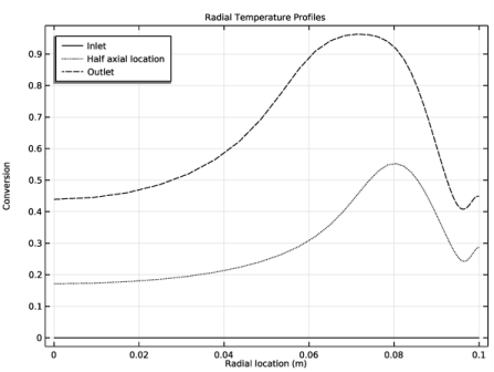
In the Settings window for Line Graph, click Replace Expression in the upper-right corner of the y-Axis Data section. From the menu, choose Component 1 (comp1)>Definitions>Variables>xA - Conversion species A.
|
|
1
|
|
2
|
|
3
|
|
4
|
|
1
|
|
2
|
|
1
|
|
2
|
|
3
|
|
4
|
|
5
|
|
1
|
|
2
|
|
1
|
|
2
|
|
3
|