Pacemaker Electrode

This example illustrates the use of COMSOL Multiphysics for modeling of ionic current distribution problems in electrolytes, in this case in human tissue. The problem is exemplified on a pacemaker electrode, but it can be applied in electrochemical cells like fuel cells, batteries, corrosion protection, or any other process where ionic conduction takes place in the absence of concentration gradients.

The modeled device is a pacemaker electrode that is placed inside the heart and helps the patient’s heart to keep a normal rhythm. The device is referred to as an electrode, but it actually consists of two electrodes: a cathode and an anode.

Figure 1 shows a schematic drawing of two pair of electrodes placed inside the heart. The electrodes are supplied with current from the pulse generator unit, which is also implanted in the patient.

Figure 1: Schematic drawing of the heart with two pairs of pacemaker electrodes.

This example deals with the current and potential distribution around one pair of electrodes.

Model Definition

The model domain consists of the blood and tissue surrounding the electrode pair. The actual electrodes and the electrode support are boundaries to the modeled domain. Figure 2 shows the electrode in a darker shade, while the surrounding modeling domain is shown in a lighter shade.

Figure 2: Modeling domain and boundaries.

The working electrode consists of a hemisphere placed on the tip of the supporting cylindrical structure. The counter electrode is placed in the “waist” of this structure. All other surfaces of the supporting structure are insulated. The outer boundaries are placed far enough from the electrode to give a small impact on the current and potential distribution.

In COMSOL Multiphysics, use the Electric Currents interface for the analysis of the electrode. This physics interface is useful for modeling conductive materials where a current flows due to an applied electric field.

Domain Equations

The current in the domain is controlled by the continuity equation, which follows from Maxwell’s equations:

where σ is the conductivity of the human tissue. This equation uses the following relations between the electric potential and the fields.

Boundary Conditions

Ground potential boundary conditions are applied on the thinner waist of the electrode. The tip of the electrode has a fixed potential of 1 V. All other boundaries are electrically insulated.

Results and Discussion

This simulation gives the potential distribution on the electrode surface and streamlines of the current distribution inside the human heart; see Figure 3.

Figure 3: The plot shows the electrostatic potential distributed on the surface of the electrode. The total current density is shown as streamlines.

As expected, the current density is highest at the small hemisphere, which is the one that causes the excitation of the heart. The current density is fairly uniform on the working electrode. The counter electrode is larger and there are also larger variations in current density on its surface. Mainly, the current is lower with increasing distance from the working electrode. The model shows that the anchoring arms of the device have little influence on the current density distribution.

COMSOL_Multiphysics/Electromagnetics/pacemaker_electrode

Modeling Instructions

From the menu, choose .

New

In the window, click

Model Wizard

In the window, click

In the tree, select .

Click .

Click

In the tree, select .

Click

Geometry 1

Insert the geometry sequence from the pacemaker_electrode_geom_sequence.mph file.

In the toolbar, click and choose .

Browse to the model’s Application Libraries folder and double-click the file pacemaker_electrode_geom_sequence.mph.

In the toolbar, click

Next, define the volume surrounding the electrode. The simulation only takes place in this volume, where the boundaries of the electrode influence the result.

Cylinder 1 (cyl1)

In the toolbar, click

In the window for , locate the section.

In the text field, type 10[mm].

In the text field, type 40[mm].

Locate the section. In the text field, type -20[mm].

Difference 1 (dif1)

In the toolbar, click

and choose .

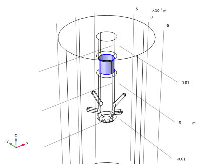
Select the object only.

In the window for , locate the section.

From the list, choose .

Form Union (fin)

In the toolbar, click

Definitions

Next, define a selection corresponding to the grounded electrode for later use.

Geometry 1

Counter Electrode

In the toolbar, click

and choose .

In the window for , locate the section.

From the list, choose .

Select the check box.

Click the

button in the toolbar.

On the object , select Boundaries 29, 30, 58, and 63 only.

In the text field, type Counter Electrode.

Click the

button in the toolbar to restore the default rendering state.

Materials

A convenient way to find out which material parameters you need to specify is to add a material. COMSOL Multiphysics then indicates any missing parameters for the physics interfaces you have added to the model.

Heart Tissue

In the window, under right-click and choose .

By default, the first material you add applies to all domains, so you do not need to modify the geometric scope.

The electrode is inserted into the human heart, so you must specify the conductivity for the heart tissue.

In the window for , locate the section.

In the table, enter the following settings:


Property	Variable	Value	Unit	Property group
Electrical conductivity	sigma_iso ; sigmaii = sigma_iso, sigmaij = 0	0.4[S/m]	S/m	Basic
Relative permittivity	epsilonr_iso ; epsilonrii = epsilonr_iso, epsilonrij = 0	1	1	Basic

In the text field, type Heart Tissue.

Electric Currents (ec)

The only physics settings that remain to specify are the electrode potentials.

Ground 1

In the window, under right-click and choose .

In the window for , locate the section.

From the list, choose .

Electric Potential 1

In the toolbar, click

and choose .

In the window for , locate the section.

From the list, choose .

Locate the section. In the V0 text field, type 1.

Mesh 1

Use the default physics-controlled mesh.

In the window, under right-click and choose .

Study 1

Use the default settings for the stationary solver, which gives the conjugate gradients iterative solver with algebraic multigrid as the preconditioner.

In the toolbar, click

Results

Electric Potential (ec)

The default plot shows the slices of the electrical potential. To reproduce the plot shown in Figure 3, start by hiding the outer boundaries.

Electric Currents (ec)

In the window, under click .

Click the

button in the toolbar.

In the window toolbar, click

next to

, then choose .

Select Boundaries 1–4, 45, and 74 only.

Click the

button in the toolbar.

Results

3D Plot Group 3

In the toolbar, click

and choose .

In the window for , locate the section.

Clear the check box.

Surface 1

Right-click and choose .

In the toolbar, click

3D Plot Group 3

Combine the surface plot of the potential with streamlines visualizing the total current density.

Streamline 1

In the window, right-click and choose .

In the window for , locate the section.

From the list, choose .

Locate the section. From the list, choose .

Locate the section. Find the subsection. From the list, choose .

In the text field, type min(ec.normJ/0.1[mA/mm^2],1)*0.2[mm]. ec.normJ is the variable for the current density norm. This expression states that tubes are 0.2[mm] wide in the points having 0.1[mA/mm^2]. The "min" function saturates the increase of the tube radius where current density approaches 0.1[mA/mm^2].

To get suitably thick streamlines you need to adjust the scale factor.

Select the check box.

In the toolbar, click

Color Expression 1

Right-click and choose .

Use the default expression. Because it is the same as the surface expression, you can disable the color legend:

In the window for , locate the section.

Clear the check box.

After proper rotation and zoom operations, you should see something similar to the plot in Figure 3.