Light Bulb Geometry

In COMSOL Multiphysics you can easily create complex two-dimensional shapes by drawing directly in the graphics window. After drawing an initial sketch, the geometry nodes corresponding to the individual components of the drawn curves can be edited to adjust the shape or to introduce parameters in the size expressions. You may also freely combine the shapes you have drawn by joining them with Boolean operations.

In this tutorial, you will create the cross section of a light bulb inside a 2D axisymmetric model component. You will first sketch the outline of the geometry and then modify the elements of the composite curves to obtain the desired shape. In addition, you will use named selections to create the selections for setting up the physics.

The step-by-step instructions demonstrate how to draw the geometry in Sketch mode, while following a workflow typical of creating geometry in COMSOL Multiphysics. Read on to find out more about the following topics:

•

How to draw 2D shapes with the drawing tools, and how to edit the resulting geometry nodes

•

How to partition an edge to create additional boundaries for the physics setup

•

How to unite the created geometry objects to form the final geometry for the simulation

•

How to set up selections that make the definition of physics settings more efficient

The multiphysics analysis of the light bulb is described in the Free Convection in a Light Bulb model located in the Heat Transfer Module Application Library.

Model Definition

The geometry you are going to create in this tutorial is the cross section of a light bulb, see Figure 1, used in the model Free Convection in a Light Bulb in the Heat Transfer Module Application Library. The outer silhouette and inner structure are created using two composite curves. In the geometry sequence you will also set up the selections for assigning the material and physics definitions.

Figure 1: Cross section of a light bulb.

This example describes only the process of creating the geometry sequence. For the physics setup, follow the instructions in Free Convection in a Light Bulb in the Heat Transfer Module Application Library.

COMSOL_Multiphysics/Geometry_Tutorials/light_bulb_geometry

Modeling Instructions

From the menu, choose .

New

In the window, click

Add Component

In the toolbar, click

and choose .

Geometry 1

In the window for , locate the section.

From the list, choose .

Begin by drawing a rough outline of the bulb. Don’t worry about getting it exactly right as you will adjust it later.

The dimensions of the light bulb are larger than the default zoom level in the Graphics window. Adjusting the shape is easier if the original sketch is drawn closer to the final size, so you can start by zooming out a few steps.

Composite Curve 1 (cc1)

In the toolbar, click , then in the window place the first vertex by clicking on the centerline close to the top of the canvas.

Move the pointer to the right, and at the end of the first horizontal segment click once to place a vertex.

To switch drawing a Cubic Bézier polygon, right-click and from the context menu choose .

Place the two control points of the Bézier curve, followed by the vertex at the end by clicking once on the canvas for each point.

To switch drawing a circular arc, right-click in the window, and from the context menu choose , then choose .

Place the center of the arc on the centerline, then move the pointer to draw the arc, and click to place the end vertex so that the arc finishes at the centerline.

Right-click, then from the context menu choose .

To close the shape, position the pointer on top of the first vertex, then click to place the last vertex. The shape will be closed automatically.

When done, the node is added to the geometry sequence. This node contains the polygon, cubic Bézier, and circular arc features that you have drawn. Note that the two adjacent straight segments are automatically combined into one feature.

Composite Curve 1 (cc1)

Next adjust the features inside to obtain the outer shape of the light bulb.

Polygon 1 (pol1)

In the window, expand the node, then click .

In the window for , locate the section.

In the table, enter the following settings:


r (mm)	z (mm)
0	-25
0	42
10	42

When editing the coordinates of the features in a , the adjacent features are automatically updated to keep the start and end points of adjacent edges are coincident.

Cubic Bézier 1 (cb1)

In the window, click .

In the window for , locate the section.

In row , set to 18.

In row , set to 41.

In row , set to 13*sqrt(2).

In row , set to 13*sqrt(2)+1.

Circular Arc 1 (ca1)

In the window, click .

In the window for , locate the section.

In the text field, type 0.

In the text field, type 1.

Locate the section. In the text field, type 26.

Locate the section. In the text field, type 45.

In the text field, type -90.

Click

Composite Curve 1 (cc1)

In the window, click .

In the window for , locate the section.

Select the check box.

From the list, choose . With this setting the selection is available only as input for features in the geometry sequence. This way you can keep only the relevant selections in the list of selections when you are defining, for example, physics and mesh features.

Partition Edges 1 (pare1)

In the toolbar, click

and choose .

On the object , select Boundary 3 only.

The partitioning operations can be useful in many cases. Here, we are partitioning the selected edge to create segments that reflect that a portion of the upper boundaries of the bulb are covered by a cap.

In the window for , click

Composite Curve 2 (cc2)

Continue with creating the interior boundaries. Draw a rough outline by starting again from the top left corner, then continuing clockwise.

Use the drawing tools in the following order:

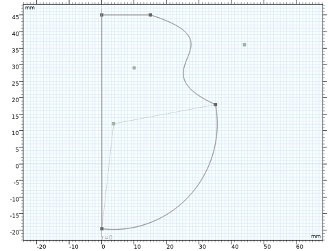
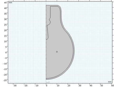
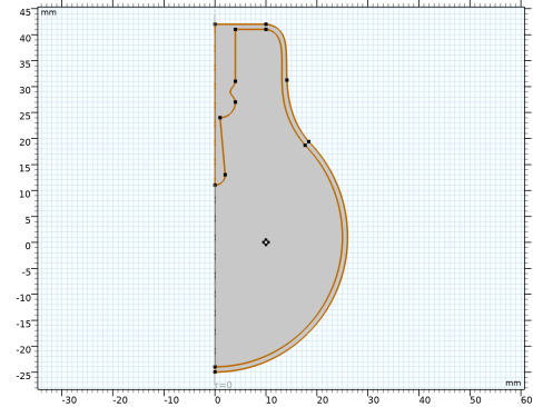
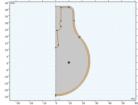
Start with a to draw an edge perpendicular to the rotation axis. Its first vertex is located inwards from the start vertex of the outer shape.

Continue with a Bézier polygon. Try to follow the outer shape.

Add a that ends on the centerline.

Draw a up along the centerline to about halfway up the geometry.

Continue with a that curves away from the centerline.

Use the tool to draw an edge that tilts towards the centerline.

Draw another that curves away from then back towards the centerline. The start and end vertices can be aligned vertically.

Switch to an to create a curved segment that first curves towards the centerline then away. Use the option to define the curve, and add one interpolation point. Try to align the start and end vertices vertically.

Close the shape with a vertical edge, using the tool.

Composite Curve 2 (cc2)

Continue with editing the features inside .

Polygon 1 (pol1)

In the window, expand the node, then click .

In the window for , locate the section.

In the table, enter the following settings:


r (mm)	z (mm)
4	31
4	41
10	41

Cubic Bézier 1 (cb1)

In the window, click .

In the window for , locate the section.

In row , set to 18.

In row , set to 40.

In row , set to 9.

In row , set to 29.

In row , set to 12.5*sqrt(2).

In row , set to 12.5*sqrt(2)+1.

Locate the section. In the text field, type 3/4.

Polygon 2 (pol2)

In the window, click .

In the window for , locate the section.

In the table, enter the following settings:


r (mm)	z (mm)
0	11

Circular Arc 2 (ca2)

In the window, click .

In the window for , locate the section.

In the text field, type 13.

Locate the section. In the text field, type 2.

Polygon 3 (pol3)

In the window, click .

In the window for , locate the section.

In the table, enter the following settings:


r (mm)	z (mm)
1	24

Circular Arc 3 (ca3)

In the window, click .

In the window for , locate the section.

In the text field, type 1.

In the text field, type 27.

Locate the section. In the text field, type 3.

Locate the section. In the text field, type -90.

In the text field, type 0.

Interpolation Curve 1 (ic1)

In the window, click .

In the window for , locate the section.

In the table, enter the following settings:


r (mm)	z (mm)
3	29
4	31

Locate the section. From the list, choose .

In the text field, type 0.

In the text field, type 1.

From the list, choose .

In the text field, type 0.

In the text field, type 1.

Composite Curve 2 (cc2)

In the window, click .

In the window for , click

Locate the section. Select the check box.

From the list, choose .

Tungsten

In the toolbar, click

In the window for , type Tungsten in the text field.

Locate the section. In the text field, type 0.5.

Locate the section. In the text field, type 10.

Locate the section. Select the check box.

From the list, choose .

Click

The geometry is finished, but before continuing let’s leave Sketch mode, and inspect the geometry using the window.

In the toolbar, click

and choose .

Selection List

Go to the window.

Here you can view a list of geometric objects and entities, and named selections, that exist in the geometry at the current build state for the selected entity level. The list on the top contains objects and entities, and the one at the bottom displays the named selections.

Let’s take a look at the three objects that comprise the geometry.

In the window toolbar, click

next to

, then choose .

Go to the window.

In the tree, select .

In the tree, select .

In the tree, select .

The domains for the glass, and the Argon gas, and the Tungsten filament result after geometric Boolean operations of these three objects. Namely, the domain for the glass is the difference of the Composite Curve 1 and Composite Curve 2 objects, and the domain for the Argon gas is the difference of the Composite Curve 2 and Tungsten objects.

Fortunately, COMSOL Multiphysics automatically computes these domains in the Form Union operation, which is at the end of the geometry sequence, and creates the union of all geometry objects that exist in the sequence while preserving interior boundaries to separate domains.

Geometry 1

Form Union (fin)

In the window, under click .

In the window for , click

After , only one object is displayed in the upper list of the window. This finalized geometry is divided into domains along the boundaries of the initial objects.

In the window toolbar, click