PDF

Automotive Muffler
Introduction
This example describes the pressure wave propagation in a muffler for an explosion engine. The approach is general for analysis of damping of harmonic pressure waves.
The purpose of the application is to show how to treat 3D acoustics in a fairly complex geometry consisting of several separate sections and pipes divided by thin perfectly rigid walls. The analysis gives the transmission loss in the frequency range 100 Hz–1000 Hz.
Model Definition
The model geometry consists of three separate resonator chambers divided by thin walls. The inlet and the outlet correspond to the connection in the direction of the engine and of free air, respectively.
Figure 1: The geometry of a muffler. The exhaust fumes enter through the left pipe, pass the three resonator chambers, and exit through the right pipe.
Domain Equations
You solve the problem in the frequency domain using the Pressure Acoustics, Frequency Domain interface. The model equation is a slightly modified Helmholtz equation for the acoustic pressure p:
where ρ is the density, c is the speed of sound, and ω is the angular frequency. The density needs to be included in the equation in cases where variations in density in different materials exist. The model assumes that in the low-frequency range, reactive damping prevails. Resistive damping is therefore not included.
Boundary Conditions
The boundary conditions are of three different types. At all the solid boundaries, which include the outer walls of the muffler, the dividing walls between the resonator chambers, and the walls of the pipes, sound hard (wall) boundary conditions are used:
At the inlet boundary, a combination of an incoming and an outgoing plane waves is assumed:
In this equation p0 denotes the applied outer pressure and i the imaginary unit. At the outlet boundary, an outgoing plane wave is set:
Results and Discussion
Figure 2 visualizes the pressure field in the muffler at a frequency of 490 Hz using a boundary plot of the absolute value of the pressure and an isosurface plot of the pressure.
Figure 2: The solution at 490 Hz. The real value of the pressure is plotted as isosurfaces, and the absolute value of the pressure is displayed as a boundary plot on the inner walls of the muffler.
The following equation defines the transmission loss in the muffler:
Here, Pin and Pout denote the acoustic effect at the inlet and outlet, respectively. The acoustic effect is calculated using the following equations:
Figure 3 shows the result of a parametric frequency study. This plot reveals that the damping is better at higher frequencies, with the exception of several deep dips throughout the frequency range. The dips correspond to the resonance frequencies for different parts of the muffler system.
Figure 3: The damping (dB) in the muffler as a function of the frequency (Hz).
Application Library path: COMSOL_Multiphysics/Acoustics/automotive_muffler
Modeling Instructions
From the File menu, choose New.
New
In the New window, click  Model Wizard.
Model Wizard
1
In the Model Wizard window, click  3D.
2
In the Select Physics tree, select Acoustics>Pressure Acoustics>Pressure Acoustics, Frequency Domain (acpr).
3
Click Add.
4
Click  Study.
5
In the Select Study tree, select General Studies>Frequency Domain.
6
Global Definitions
Parameters 1
1
In the Model Builder window, under Global Definitions click Parameters 1.
2
In the Settings window for Parameters, locate the Parameters section.
3
Geometry 1
Create the geometry. To simplify this step, insert a prepared geometry sequence.
1
In the Geometry toolbar, click Insert Sequence and choose Insert Sequence.
2
3
In the Geometry toolbar, click  Build All.
4
Click the  Zoom Extents button in the Graphics toolbar.
Definitions
Define integration operators for the inlet and outlet, then use these to calculate the attenuation.
Inlet
1
In the Definitions toolbar, click  Nonlocal Couplings and choose Integration.
2
In the Settings window for Integration, locate the Source Selection section.
3
From the Geometric entity level list, choose Boundary.
4
5
In the Operator name text field, type intop_inlet.
6
In the Label text field, type Inlet.
Outlet
1
In the Definitions toolbar, click  Nonlocal Couplings and choose Integration.
2
In the Settings window for Integration, locate the Source Selection section.
3
From the Geometric entity level list, choose Boundary.
4
Click the  Wireframe Rendering button in the Graphics toolbar.
5
6
In the Operator name text field, type intop_outlet.
7
In the Label text field, type Outlet.
Variables 1
1
In the Definitions toolbar, click  Local Variables.
2
In the Settings window for Variables, locate the Variables section.
3
Note that you need to define the incoming power using p0 rather than the pressure variable, p, because p is the sum of incident and reflected pressure waves.
Interior Boundaries
Create a selection to simplify setting up the interior boundary conditions.
1
In the Definitions toolbar, click  Explicit.
2
In the Settings window for Explicit, locate the Input Entities section.
3
From the Geometric entity level list, choose Boundary.
4
To do this, click the Paste Selection button next to the Selection box, paste the text: 10, 11, 13, 14, 16, 20–23, 25, 26, 28, 29, 32, 36–39 in the text field of the dialog box that opens, and finally click OK.
5
Click the  Wireframe Rendering button in the Graphics toolbar to return to the original state.
6
In the Label text field, type Interior Boundaries.
Add Material
1
In the Home toolbar, click  Add Material to open the Add Material window.
2
Go to the Add Material window.
3
4
Click Add to Component in the window toolbar.
5
In the Home toolbar, click  Add Material to close the Add Material window.
Materials
By default, the first material you add applies for all domains. In the Material Contents table you can see which material properties the physics interfaces use, in this case the density and the speed of sound. Notice that these quantities are functions of the temperature and (in the case of the density) the ambient pressure.
Pressure Acoustics, Frequency Domain (acpr)
Pressure Acoustics 1
In the Model Inputs section you can read off and, if desired, modify the temperature and absolute pressure at which the expressions for the air density and speed of sound are calculated. For this model, use the default settings.
Plane Wave Radiation 1
1
In the Model Builder window, right-click Pressure Acoustics, Frequency Domain (acpr) and choose Radiation Conditions>Plane Wave Radiation.
2
Incident Pressure Field 1
1
In the Physics toolbar, click  Attributes and choose Incident Pressure Field.
2
In the Settings window for Incident Pressure Field, locate the Incident Pressure Field section.
3
In the p0 text field, type p0.
4
From the c list, choose From material.
5
From the Material list, choose Air (mat1).
Plane Wave Radiation 2
1
In the Physics toolbar, click  Boundaries and choose Plane Wave Radiation.
2
Note that the Plane Wave Radiation boundary condition is only suitable for plane waves at near right angles of incidence. For general types of waves in waveguides, use the Port boundary condition available with the Acoustics Module as shown in the Absorptive Muffler tutorial model.
3
Click the  Transparency button in the Graphics toolbar to return to the default transparency state.
Interior Sound Hard Boundary (Wall) 1
1
In the Physics toolbar, click  Boundaries and choose Interior Sound Hard Boundary (Wall).
2
In the Settings window for Interior Sound Hard Boundary (Wall), locate the Boundary Selection section.
3
From the Selection list, choose Interior Boundaries.
Mesh
Proceed and generate the mesh using the Physics-controlled mesh functionality. The frequency controlling the maximum element size is per default taken From study. Set the desired Frequencies in the study step. In general, 5 to 6 second-order elements per wavelength are needed to resolve the waves. For more details, see Meshing (Resolving the Waves) in the Acoustics Module User’s Guide. In this model, we use 10 elements per wavelength; the default Automatic is to have 5.
Study 1
Step 1: Frequency Domain
1
In the Model Builder window, under Study 1 click Step 1: Frequency Domain.
2
In the Settings window for Frequency Domain, locate the Study Settings section.
3
In the Frequencies text field, type range(100,10,1000).
This computes the solution for 91 equally spaced frequencies from 100 Hz to 1000 Hz. If you want to run a faster analysis, try the same frequency range but with a step of 100 Hz instead (to do so, type range(100,100,1000)).
Mesh 1
1
In the Model Builder window, under Component 1 (comp1) click Mesh 1.
2
In the Settings window for Mesh, locate the Pressure Acoustics, Frequency Domain (acpr) section.
3
From the Number of mesh elements per wavelength list, choose User defined.
4
5
Click  Build All.
Study 1
In the Home toolbar, click  Compute.
Results
Before visualizing the acoustic pressure field, add a selection to the default solution dataset that filters out the upper muffler boundaries for a better view.
Study 1/Solution 1 (sol1)
In the Model Builder window, expand the Results>Datasets node, then click Study 1/Solution 1 (sol1).
Selection
1
In the Results toolbar, click  Attributes and choose Selection.
2
In the Settings window for Selection, locate the Geometric Entity Selection section.
3
From the Geometric entity level list, choose Boundary.
4
Choose All boundaries from the Selection list.
5
Alternatively, you can click the Paste Selection button next to the Selection box and then paste the text “1–7, 9–14, 16, 17, 19–29, 31–33, 35–41, and 43–50” in the text field of the dialog box that opens before clicking OK.
Acoustic Pressure (acpr)
Reproduce the plot in Figure 2 by following these steps.
1
In the Model Builder window, under Results click Acoustic Pressure (acpr).
2
In the Settings window for 3D Plot Group, locate the Data section.
3
From the Parameter value (freq (Hz)) list, choose 490.
Surface 1
1
In the Model Builder window, expand the Acoustic Pressure (acpr) node, then click Surface 1.
2
In the Settings window for Surface, click Replace Expression in the upper-right corner of the Expression section. From the menu, choose Component 1 (comp1)>Pressure Acoustics, Frequency Domain>Pressure and sound pressure level>acpr.absp_t - Absolute total acoustic pressure - Pa.
3
Locate the Coloring and Style section. From the Scale list, choose Linear.
4
In the Acoustic Pressure (acpr) toolbar, click  Plot.
Isosurface 1
1
In the Model Builder window, right-click Acoustic Pressure (acpr) and choose Isosurface.
2
In the Settings window for Isosurface, click Replace Expression in the upper-right corner of the Expression section. From the menu, choose Component 1 (comp1)>Pressure Acoustics, Frequency Domain>Pressure and sound pressure level>p - Pressure - Pa.
3
Locate the Levels section. In the Total levels text field, type 10.
4
Locate the Coloring and Style section. Click  Change Color Table.
5
In the Color Table dialog box, select Wave>Wave in the tree.
6
7
In the Settings window for Isosurface, locate the Coloring and Style section.
8
From the Scale list, choose Linear symmetric.
What is a suitable number of isosurface levels for the isosurface plot varies with the frequency. At frequencies with low damping many of the isosurfaces tend to congregate inside the pipe.
9
In the Acoustic Pressure (acpr) toolbar, click  Plot.
10
Click the  Zoom Extents button in the Graphics toolbar.
Finally, reproduce the plot of attenuation versus frequency shown in Figure 3.
1D Plot Group 4
In the Home toolbar, click  Add Plot Group and choose 1D Plot Group.
Global 1
1
Right-click 1D Plot Group 4 and choose Global.
2
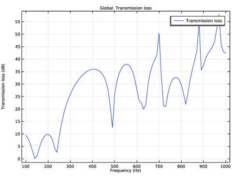
In the Settings window for Global, click Replace Expression in the upper-right corner of the y-Axis Data section. From the menu, choose Component 1 (comp1)>Definitions>Variables>TL - Transmission loss.
Transmission Loss
1
In the Model Builder window, under Results click 1D Plot Group 4.
2
In the Settings window for 1D Plot Group, type Transmission Loss in the Label text field.
3
Locate the Plot Settings section.
4
Select the x-axis label check box. In the associated text field, type Frequency (Hz).
5
Select the y-axis label check box. In the associated text field, type Transmission loss (dB).
6
In the Transmission Loss toolbar, click  Plot.
Notice the deep dip in the damping around 490 Hz caused by the resonance in the second chamber. If you plot the pressure in the muffler at other dips, resonances in the other chambers appear.