PDF

Adsorption and Desorption of Water in a Load Lock Vacuum System
Introduction
This model shows how to simulate the time-dependent adsorption and desorption of water in a vacuum system at low pressures. The water is introduced into the system when a gate valve to a load lock is opened and the subsequent migration and pumping of the water is modeled.
Model Definition
The model geometry is shown in Figure 1. The system consists of two chambers separated by a gate valve (not shown in the geometry). The lower cylindrical chamber is the load lock chamber. The upper spherical chamber is a high vacuum chamber, which is not vented during the sample loading process. The vacuum pump is located opposite the gate valve, and has a constant speed of 500 l/s.
Figure 1: Axisymmetric model geometry, shown in 2D (left) and 3D (right).
Water Adsorption and Desorption
Several simplifying assumptions are made about the adsorption and desorption of the water vapor in this model:
The density of the water adsorption sites is assumed to be 1 × 10-4 mol/m2. This corresponds to 6 × 1015 molecules/cm2, consistent with typical outgassing data reported in Ref. 2.
It is assumed that the water does not dissociate when adsorbing, so that the desorption process is first order (the desorption rate is therefore proportional to the molar concentration of adsorbed molecules, nads). Since the flow is isothermal, the desorption rate, D, is determined by a constant time constant, τ (D=nads/τ). τ is chosen as 200 s to produce reasonable agreement with the outgassing data reported in Ref. 2 and with the range of data reported in Ref. 1.
COMSOL Multiphysics treats the adsorption and desorption of molecules in a molecular flow by specifying a sticking coefficient (S) and a molar desorption rate (D) such that:
(1)
where J is the emitted molecular flux, G is the incident molecular flux, NA is Avogadro’s number and Γ is an additional surface source of molar flux (enabling, for example, the coupling of a diffusion problem to the interface in order to model the diffusion or permeation of gases through the walls of the system). An initial value is specified for nads on each surface.
In this model the sticking coefficient S is given the following value:
(2)
where S0 is the sticking coefficient with no site occupancy (assumed to be 0.1) and nsites is the molar capacity of the surface sites on the system (assumed to be 1 × 10-4 mol/m2). The model sets the desorption rate in the following manner:
(3)
where τ is the time constant for desorption. Equation 3 assumes that the desorption process is first order, that is that there is no dissociation of the water on adsorption, or recombination required for desorption.
The wall boundary condition implements Equation 1 automatically when the Adsorption/Desorption wall type is selected. Equation 2 and Equation 3 are implemented with expressions typed into the boundary condition. S0 (sc), nsites (nsites) and τ (tau) are all parameters in the model with the names indicated in the brackets.
Results and Discussion
Figure 2 shows the evolution of the adsorbed molecules per unit area on the surface of the system, as the water vapor is pumped out. A redistribution of the molecules between the load lock and the high vacuum chamber is observed initially. After that the distribution of molecules appears qualitatively similar but the number of molecules adsorbed decreases progressively.
Figure 3 and Figure 4 show the pressure and the adsorbed molecules per unit area evolving over time as the water is pumped out. The results are shown for two points, one in the high vacuum system and the other in the load lock. The two curves are similar in form. Initially the pressure in the load lock is significantly higher than that in the high vacuum system. After approximately 0.3 hours (18 mins) the pressure in the two parts of the system converges and there is a smaller, time independent difference between the pressure measured in the two chambers. For the first three hours of pumping the pressure in the system drops slowly, but after that a more rapid decrease in the pressure occurs as the remainder of the water is pumped out. Using the load lock ensures that the pressure in the high vacuum part of the system remains below 7 × 10-7 Torr.
Figure 2: Molecules adsorbed per square meter on the surface of the chamber as a function of time.
Figure 3: Pressure as a function of time at points in the load lock and high vacuum chambers.
Figure 4: Adsorbed molecules per unit area at points in the load lock and high vacuum chambers.
Application Library path: Molecular_Flow_Module/Industrial_Applications/water_adsorption_desorption
References
1. J.F. O’Hanlon, A User’s Guide to Vacuum Technology, John Wiley & Sons, 2003.
2. H.F. Dylla, “The Problem of Water in Vacuum Systems”, CERN Accelerator School, Platja d’Aro, Spain, May 2006 (available at: http://cas.web.cern.ch/sites/cas.web.cern.ch/files/lectures/platjadaro-2006/dylla-2.pdf).
3. J.M. Lafferty, Foundations of Vacuum Science and Technology, John Wiley & Sons, 1998.
Modeling Instructions
From the File menu, choose New.
New
In the New window, click  Model Wizard.
Model Wizard
1
In the Model Wizard window, click  2D Axisymmetric.
2
In the Select Physics tree, select Fluid Flow>Rarefied Flow>Free Molecular Flow (fmf).
3
Click Add.
4
In the Incident molecular fluxes table, enter the following settings:
5
Click  Study.
6
In the Select Study tree, select General Studies>Time Dependent.
7
Global Definitions
Parameters 1
1
In the Model Builder window, under Global Definitions click Parameters 1.
2
In the Settings window for Parameters, locate the Parameters section.
3
Geometry 1
Circle 1 (c1)
1
In the Geometry toolbar, click  Circle.
2
In the Settings window for Circle, locate the Size and Shape section.
3
In the Radius text field, type 16[in].
4
In the Sector angle text field, type 180.
5
Locate the Rotation Angle section. In the Rotation text field, type 270.
Rectangle 1 (r1)
1
In the Geometry toolbar, click  Rectangle.
2
In the Settings window for Rectangle, locate the Size and Shape section.
3
In the Width text field, type 14[in].
4
In the Height text field, type 22[in].
5
Locate the Position section. In the z text field, type -46[in].
Rectangle 2 (r2)
1
In the Geometry toolbar, click  Rectangle.
2
In the Settings window for Rectangle, locate the Size and Shape section.
3
In the Width text field, type 7.5[in].
4
In the Height text field, type 70[in].
5
Locate the Position section. In the z text field, type -50[in].
Point 1 (pt1)
1
In the Geometry toolbar, click  Point.
2
In the Settings window for Point, locate the Point section.
3
In the r text field, type 7.5[in].
4
In the z text field, type -20[in].
Union 1 (uni1)
1
In the Geometry toolbar, click  Booleans and Partitions and choose Union.
2
Select the objects c1, r1, and r2 only.
3
In the Settings window for Union, locate the Union section.
4
Clear the Keep interior boundaries check box.
Rectangle 3 (r3)
1
In the Geometry toolbar, click  Rectangle.
2
In the Settings window for Rectangle, locate the Size and Shape section.
3
In the Width text field, type 1.5[in].
4
In the Height text field, type 50[in].
5
Locate the Position section. In the z text field, type -50[in].
Compose 1 (co1)
1
In the Geometry toolbar, click  Booleans and Partitions and choose Compose.
2
Select the objects r3 and uni1 only.
3
In the Settings window for Compose, locate the Compose section.
4
In the Set formula text field, type uni1-r3.
5
Click  Build Selected.
6
Click the  Zoom Extents button in the Graphics toolbar.
Free Molecular Flow (fmf)
Molecular Flow 1
1
In the Model Builder window, under Component 1 (comp1)>Free Molecular Flow (fmf) click Molecular Flow 1.
2
In the Settings window for Molecular Flow, locate the Molecular Weight of Species section.
3
In the Mn,H2O text field, type 0.018[kg/mol].
Wall 1
1
In the Model Builder window, click Wall 1.
2
In the Settings window for Wall, locate the Wall Type section.
3
From the Wall type list, choose Adsorption/Desorption.
4
Locate the Adsorption/Desorption section. In the SH2O text field, type sc*(1-fmf.n_ads_H2O/nsites).
5
In the DH2O text field, type fmf.n_ads_H2O/tau.
6
In the nads,0,H2O text field, type 0.
Wall 2
1
Right-click Component 1 (comp1)>Free Molecular Flow (fmf)>Wall 1 and choose Duplicate.
2
3
In the Settings window for Wall, locate the Adsorption/Desorption section.
4
In the nads,0,H2O text field, type nsites.
Vacuum Pump 1
1
In the Physics toolbar, click  Boundaries and choose Vacuum Pump.
2
3
In the Settings window for Vacuum Pump, locate the Vacuum Pump section.
4
From the Specify pump flux list, choose Pump speed.
Mesh 1
Edge 1
1
In the Mesh toolbar, click  Edge.
2
In the Settings window for Edge, locate the Boundary Selection section.
3
From the Selection list, choose All boundaries.
Size
1
In the Model Builder window, click Size.
2
In the Settings window for Size, locate the Element Size section.
3
From the Predefined list, choose Extra fine.
4
Click  Build All.
Study 1
Step 1: Time Dependent
1
In the Model Builder window, under Study 1 click Step 1: Time Dependent.
2
In the Settings window for Time Dependent, locate the Study Settings section.
3
In the Output times text field, type range(0,100,1000) range(2000,1000,10000) 1e4*10^{range(0,0.1,1)}.
Use several ranges for the time steps, to obtain good resolution on different time scales.
Reduce the relative and absolute solver tolerance by an order of magnitude. This is recommended as the number of adsorbed molecules varies over several orders of magnitude.
4
From the Tolerance list, choose User controlled.
5
In the Relative tolerance text field, type 0.0001.
Solution 1 (sol1)
1
In the Study toolbar, click  Show Default Solver.
2
In the Model Builder window, expand the Solution 1 (sol1) node, then click Time-Dependent Solver 1.
3
In the Settings window for Time-Dependent Solver, click to expand the Absolute Tolerance section.
4
From the Tolerance method list, choose Manual.
5
In the Absolute tolerance text field, type 0.00001.
6
In the Study toolbar, click  Compute.
Results
Adsorbed Molecules
1
In the Home toolbar, click  Add Plot Group and choose 3D Plot Group.
2
In the Settings window for 3D Plot Group, type Adsorbed Molecules in the Label text field.
Surface 1
1
Right-click Adsorbed Molecules and choose Surface.
2
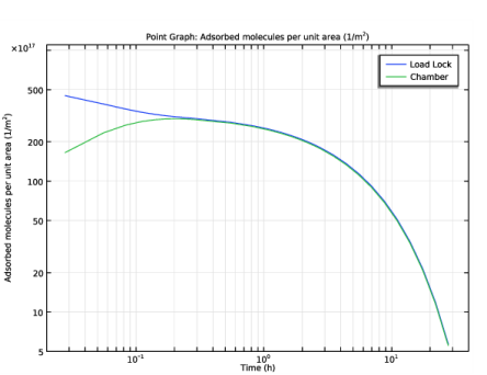
In the Settings window for Surface, click Replace Expression in the upper-right corner of the Expression section. From the menu, choose Component 1 (comp1)>Free Molecular Flow>Adsorbed/Deposited species>fmf.N_ads_H2O - Adsorbed molecules per unit area - 1/m².
3
Locate the Coloring and Style section. Click  Change Color Table.
4
In the Color Table dialog box, select Thermal>Plasma in the tree.
5
6
In the Adsorbed Molecules toolbar, click  Plot.
Compare the resulting plot with Figure 2 at different time steps.
Pressure vs. Time
1
In the Home toolbar, click  Add Plot Group and choose 1D Plot Group.
2
In the Settings window for 1D Plot Group, type Pressure vs. Time in the Label text field.
3
Locate the Axis section. Select the Manual axis limits check box.
4
In the x minimum text field, type 0.02.
5
In the x maximum text field, type 40.
6
In the y minimum text field, type 4e-9.
7
In the y maximum text field, type 1.8e-6.
8
Select the x-axis log scale check box.
9
Select the y-axis log scale check box.
Point Graph 1
1
Right-click Pressure vs. Time and choose Point Graph.
2
3
In the Settings window for Point Graph, locate the y-Axis Data section.
4
In the Expression text field, type fmf.ptot.
5
In the Unit field, type torr.
6
Locate the x-Axis Data section. From the Parameter list, choose Expression.
7
In the Expression text field, type t.
8
From the Unit list, choose h.
9
Click to expand the Legends section. Select the Show legends check box.
10
From the Legends list, choose Manual.
11
Pressure vs. Time
1
In the Model Builder window, click Pressure vs. Time.
2
In the Pressure vs. Time toolbar, click  Plot.
Compare the resulting plot with Figure 3.
Adsorbed Molecules vs. Time
1
Right-click Pressure vs. Time and choose Duplicate.
2
In the Settings window for 1D Plot Group, type Adsorbed Molecules vs. Time in the Label text field.
3
Locate the Axis section. In the y minimum text field, type 5e17.
4
In the y maximum text field, type 1.1E20.
Point Graph 1
1
In the Model Builder window, expand the Adsorbed Molecules vs. Time node, then click Point Graph 1.
2
In the Settings window for Point Graph, click Replace Expression in the upper-right corner of the y-Axis Data section. From the menu, choose Component 1 (comp1)>Free Molecular Flow>Adsorbed/Deposited species>fmf.N_ads_H2O - Adsorbed molecules per unit area - 1/m².
3
In the Adsorbed Molecules vs. Time toolbar, click  Plot.
Compare the resulting plot with Figure 4.