
|
|
|
|
1
|
|
2
|
|
3
|
Click Add.
|
|
4
|
Click
|
|
5
|
|
6
|
Click
|
|
1
|
|
2
|
Browse to the model’s Application Libraries folder and double-click the file evaporator_geom_sequence.mph.
|
|
3
|
|
4
|
|
1
|
|
2
|
|
1
|
In the Model Builder window, under Component 1 (comp1) right-click Definitions and choose Selections>Ball.
|
|
2
|
|
3
|
|
4
|
|
1
|
|
2
|
|
3
|
|
4
|
|
1
|
|
2
|
|
3
|
|
4
|
|
5
|
|
6
|
|
7
|
|
8
|
|
9
|
|
1
|
|
2
|
|
3
|
|
1
|
|
2
|
|
3
|
|
1
|
|
2
|
|
3
|
|
4
|
|
5
|
|
6
|
Click OK.
|
|
7
|
|
8
|
|
9
|
In the Add dialog box, in the Selections to subtract list, choose Boat and Shields, Front Quadrant, and Sample Mount Back.
|
|
10
|
Click OK.
|
|
1
|
|
2
|
|
3
|
|
4
|
|
5
|
Clear the Pressure check box.
|
|
1
|
In the Model Builder window, under Component 1 (comp1)>Free Molecular Flow (fmf) click Molecular Flow 1.
|
|
2
|
|
3
|
|
1
|
|
2
|
|
3
|
|
1
|
|
2
|
|
3
|
|
4
|
|
1
|
|
3
|
|
4
|
|
1
|
|
2
|
|
3
|
|
4
|
|
1
|
|
2
|
|
3
|
|
4
|
|
5
|
|
1
|
|
2
|
|
3
|
|
4
|
|
5
|
|
1
|
|
2
|
|
3
|
|
4
|
|
5
|
|
6
|
Click the Custom button.
|
|
7
|
|
8
|
|
1
|
|
2
|
|
3
|
|
4
|
|
1
|
|
2
|
|
3
|
|
4
|
|
1
|
|
2
|
|
3
|
|
4
|
|
1
|
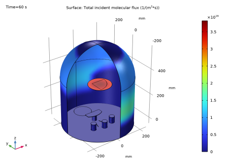
In the Model Builder window, expand the Results>Incident Molecular Flux (fmf) node, then click Surface.
|
|
2
|
|
3
|
|
1
|
|
2
|
|
1
|
|
2
|
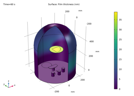
In the Settings window for Surface, click Replace Expression in the upper-right corner of the Expression section. From the menu, choose Component 1 (comp1)>Free Molecular Flow>Adsorbed/Deposited species>fmf.h_film_G - Film thickness - m.
|
|
3
|
|
4
|
|
5
|
|
6
|
Click OK.
|
|
7
|
|
8
|
|
9
|
|
10
|
|
1
|
|
2
|
|
3
|
|
1
|
|
2
|
|
1
|
|
2
|
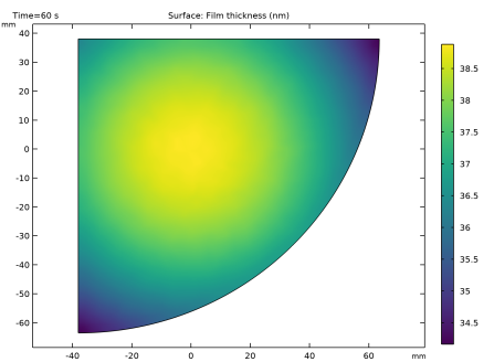
In the Settings window for Surface, click Replace Expression in the upper-right corner of the Expression section. From the menu, choose fmf.h_film_G - Film thickness - m.
|
|
3
|
|
4
|
|
5
|
|
6
|
Click OK.
|
|
7
|
|
8
|
|
9
|
|
1
|
|
2
|
|
3
|
|
4
|
|
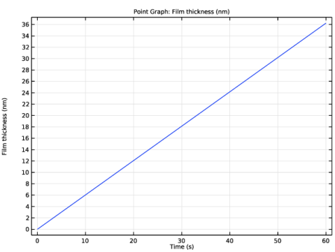
1
|
|
3
|
In the Settings window for Point Graph, click Replace Expression in the upper-right corner of the y-Axis Data section. From the menu, choose Component 1 (comp1)>Free Molecular Flow>Adsorbed/Deposited species>fmf.h_film_G - Film thickness - m.
|
|
4
|
|
5
|
|
1
|
|
2
|
|
1
|
|
2
|
|
3
|
|
4
|
|
5
|
|
6
|
|
1
|
|
2
|
|
3
|
|
4
|
|
5
|
|
1
|
|
2
|
Click in the Graphics window and then press Ctrl+A to select both objects.
|
|
3
|
|
4
|
|
1
|
|
2
|
|
3
|
|
4
|
|
5
|
|
1
|
|
2
|
|
3
|
|
4
|
|
5
|
|
6
|
|
7
|
|
1
|
|
2
|
|
3
|
|
4
|
|
5
|
Select the object cyl3 only.
|
|
6
|
|
7
|
|
1
|
|
2
|
|
3
|
|
4
|
|
5
|
|
6
|
|
7
|
|
8
|
|
9
|
|
10
|
Locate the Selections of Resulting Entities section. Find the Cumulative selection subsection. Click New.
|
|
11
|
|
12
|
Click OK.
|
|
1
|
|
2
|
|
3
|
|
4
|
Locate the Selections of Resulting Entities section. Find the Cumulative selection subsection. From the Contribute to list, choose Shield.
|
|
5
|
|
6
|
|
7
|
|
1
|
|
2
|
|
3
|
|
4
|
|
5
|
|
6
|
|
7
|
|
8
|
|
1
|
|
2
|
|
3
|
|
4
|
|
1
|
|
2
|
Select the object sph2 only.
|
|
3
|
|
4
|
|
1
|
|
2
|
|
3
|
|
4
|
|
5
|
|
6
|
|
7
|
|
8
|
|
1
|
|
2
|
|
3
|
|
4
|
|
5
|
|
6
|
|
1
|
|
2
|
|
3
|
|
1
|
|
2
|
|
3
|
|
4
|
On the object uni2, select Domains 1, 2, and 5 only.
|
|
1
|
|
2
|
|
3
|
|
4
|
|
1
|
|
2
|
|
3
|
|
1
|
|
2
|
|
3
|
|
4
|
On the object uni4, select Domains 2–4 and 7 only.
|
|
1
|
|
2
|
Select the object del2 only.
|
|
3
|
|
4
|
|
1
|
|
2
|
|
3
|
|
1
|
|
2
|
|
3
|
|
4
|
|
5
|
|
1
|
In the Model Builder window, under Component 1 (comp1)>Geometry 1 right-click Work Plane 1 (wp1) and choose Extrude.
|
|
2
|
|
4
|
|
1
|
|
2
|
|
3
|
|
1
|
|
2
|
|
3
|
|
4
|
|
1
|
In the Model Builder window, under Component 1 (comp1)>Geometry 1 right-click Work Plane 2 (wp2) and choose Work Plane.
|
|
2
|
|
3
|
|
1
|
|
2
|
|
3
|
|
4
|
|
5
|
|
6
|
|
7
|
|
1
|
In the Model Builder window, under Component 1 (comp1)>Geometry 1 right-click Work Plane 3 (wp3) and choose Booleans and Partitions>Difference.
|
|
2
|
Select the object uni1 only.
|
|
3
|
|
4
|
|
5
|
Select the objects blk1, cyl2, cyl3, ext1, mir1, rot1(1), rot1(2), rot1(3), uni5, wp2, and wp3 only.
|
|
1
|
|
2
|
On the object fin, select Boundaries 34 and 36 only.
|
|
1
|
|
2
|
On the object cmf1, select Boundary 1 only.
|
|
3
|
|
4
|
|
5
|
On the object cmf1, select Boundaries 18, 19, 22, 23, 39, 40, and 60 only.
|
|
1
|
|
2
|
On the object cmf2, select Boundary 1 only.
|
|
3
|
|
4
|
|
5
|
On the object cmf2, select Boundaries 36 and 38 only.
|
|
1
|
|
2
|
On the object cmf3, select Boundaries 17 and 64 only.
|
|
1
|
|
2
|
|
3
|
|
4
|
|
5
|
|
1
|
|
2
|
|
3
|
|
4
|
Select the object clf1 only.
|
|
1
|
|
2
|
|
3
|
|
4
|
|
5
|
Click OK.
|
|
6
|
|
7
|
|
1
|
|
2
|
|
3
|
|
4
|
|
5
|
|
6
|
|
7
|
Click OK.
|
|
1
|
|
2
|
|
3
|
|
4
|
On the object clf1, select Boundaries 1 and 4 only.
|
|
1
|
|
2
|
|
3
|
|
4
|
|
5
|
On the object clf1, select Boundaries 9, 10, 12, 44, and 52 only.
|
|
1
|
|
2
|
|
3
|
|
4
|
|
5
|
|
6
|
Click OK.
|
|
7
|
|
8
|
Click
|
|
9
|
In the Add dialog box, in the Selections to subtract list, choose Boat and Shields, Front Quadrant, and Sample Mount Back.
|
|
10
|
Click OK.
|
|
1
|
|
2
|
|
3
|
|
4
|
|
5
|
On the object clf1, select Boundaries 1, 2, 4, 5, 25, 42, 43, 49, 53, and 59 only.
|
|
1
|
|
2
|
|
3
|
|
4
|
On the object clf1, select Boundary 21 only.
|