You are viewing the documentation for an older COMSOL version. The latest version is available here.
PDF

Differential Pumping
Introduction
Differentially pumped vacuum systems use a small orifice or tube to connect two parts of a vacuum system at very different pressures. Such systems are necessary when processes run at higher pressures and are monitored by detectors that require UHV for operation.
In this model, the gas flow through a narrow tube connecting a high vacuum chamber to a chamber held at a lower pressure is approximated using an analytic expression for the flow rate down the tube. The flow is assumed to be isothermal (in practice this may be a rather poor assumption, but it is straightforward to adapt the model to use experimental data directly in place of the analytic expressions).
In the first study, the outgassing wall boundary condition is used at the outlet of the tube (high vacuum side) to solve the problem, meshing only one reservoir. The mass flow rate into the chamber is obtained from an analytical expression developed in Ref. 1. This approach enables the simulation of flows across a range of pressures within the tube, including instances when the flow inside the tube is transitional. It is necessarily an approximation, since, Knudsen’s cosine law is assumed to apply at the outlet, whilst in practice there is some focusing of the flow (molecular beaming) as a result of the tube.
The second study treats the case where the pressure in the high pressure reservoir is sufficiently low that flow through the entire tube is in the molecular flow regime. In this case, the tube can be simulated in addition to the high vacuum reservoir. The results obtained are compared with those obtained by the first approach in the appropriate limit.
Model Definition
Figure 1 shows a schematic representation of the model. There are two large reservoirs (named a and b) connected by a small tube of diameter D and length L. Each reservoir has its own steady state pressure defined by variables pa in a and pb in b. Reservoir b is connected to a vacuum pump and has a steady-state pressure pb that is smaller than reservoir a (pa>pb). Note that the tube has a finite length and thus, you can expect to see a difference in pressure between the reservoirs and the tube entrances; that is, pa>pa and pb>pb, where pa and pb are the inlet and outlet pressure, respectively.
In the steady state, the mass flow rate is constant in every region of the tube (entrances and central sections). Note that this model also uses the assumption of an isothermal flow (that is, a constant temperature everywhere in the system).
Figure 1: Not-to-scale schematic of the model. It consists of two large reservoirs at different pressures connected by a small tube.
First Study
In the first part of the model, the outgassing wall boundary condition is used at the outlet of the tube (on the high vacuum side, or side b) to represent the flow coming out of the tube from the low vacuum reservoir, which is held at pressure pa>pb. This approach allows a significant reduction in the problem size at the expense of some simplifying assumptions. The mass flow in the tube is obtained from the analytical expression developed in Ref. 1.
Analytical expression for the mass flow rate
For finite length tubes, the pressure difference between the two reservoirs differs from that between the corresponding entry regions (inlet/outlet) as a result of entry and exit flows. In order to determine an analytical expression for the mass flow rate, Gallis and Torczynski decomposed the tube into three regions (the inlet, the tube, and the outlet), each of them defining a resistance (B) that can be use to define the mass flow rate by treating the tube as resistances in series (Ref. 1). In terms of mass conductance (inverse of the mass resistance), the mass flow rate can be written as:
where A =1/B is the mass conductance. δp is the pressure difference, given by δp = pi, − pi, Where pi is either the inlet or outlet tube pressure. Finally, β is given by:
where D is the tube diameter, μ is the gas viscosity, and c is the molecular mean thermal speed, given by:
Here Mn is the molar mass, T is the temperature, and R is the ideal gas constant.
Assuming a constant mass flow rate through the tube one can see that the inlet and outlet mass conductances, for all flow regimes, are approximated by summing the corresponding continuum and free-molecular mass conductances. This results in the following equation:
(1)
where the variable q is defined by:
(2)
pλ is defined as the tube pressure at which the average Knudsen number is unity; that is:
From Ref. 1, the mass flow rate for an arbitrary-length tube can be approximated by:
(3)
with,
and
where α is the accommodation coefficient on the tube walls and where the coefficients b0, b1, b2, and ε are defined as:
where:
Combining Equation 1 and Equation 3, it is possible to determine the inlet and outlet pressure through Equation 2 and then to define the mass flow rate using
and
Second Study: Validation
The second study is intended to simulate the mass flow rate and inlet/outlet pressure at the tube in order to compare the results obtained with the molecular flow interface with the analytical expression from Ref. 1 when the flow within the tube is entirely free molecular. In this case both the high vacuum reservoir and the tube are included in the model. At the low pressure end of the tube, the reservoir boundary condition, which sets pa,, is used.
Model Geometry
The model geometry is shown in Figure 2. Note that only the high vacuum chamber is included in the model — the low vacuum chamber geometry does not need to be modeled in detail. In addition, the Plane Symmetry boundary condition is used, so the model geometry only shows half of the high vacuum chamber in order to save computational resources.
Figure 2: Model geometry. The high vacuum chamber is shown in full detail. The narrow tube that joins the two parts of the system is on the left side of the figure. Only the port connecting to the low vacuum chamber is shown in the figure (on the left side); the low vacuum chamber itself is not included in the geometry or the model.
Results and Discussion
Figure 3 shows the incident molecular flux on the surface of the high vacuum chamber at the lowest applied pressure. The corresponding number density is shown in Figure 4. The flux and number density distributions are similar for all parameters. This is expected since no geometrical changes have been made.
Figure 3: Incident molecular flux on the surface of the high vacuum chamber when the pressure in the low vacuum chamber (pa,inf) is 0.1 mTorr. Flow through the tube is modeled using the expressions from Ref. 1 and assuming diffuse emission from the outlet.
Figure 4: Number density on the surface of the high vacuum chamber when the pressures in the low vacuum chamber (pa,inf) is 0.1 mTorr. Flow through the tube is modeled using the expressions from Ref. 1 and assuming diffuse emission from the outlet.
A number of interesting features are apparent in Figure 3 and Figure 4. The shadowing effect of the port to which the tube is attached is apparent. Surfaces with a clear line of sight to the pump have a lower molecular flux and number density than those without a clear line of sight — consider for example the upper and lower surfaces of the port opposite the tube. The variation in the total flux is relatively small, approximately 1% of its absolute magnitude. Note that a higher integration resolution than the default is required to see this fine detail in the number density distribution.
Figure 5 shows the mass flow rate through the tube, as a function of the applied pressure. When the flow rate is normalized to the flow that would occur in an infinite tube (for which entry and exit effects can be neglected) a clear minimum in the flow rate as a function of pressure can be seen (see Figure 6). This is known as Knudsen’s minimum. The minimum is not apparent in Figure 5, due to the effect of the pump, which is assumed to have a constant pump speed and consequently produces different pressures on the high vacuum side, depending on the mass flow into this part of the chamber. The free molecular flow in the high vacuum chamber and the flow through the tube (which is potentially transitional) are coupled together by the model in a self consistent manner. Note that the analytic model for the mass flow rate assumes an isothermal flow and in practice there may be significant cooling of the gas as it flows through the tube. However the analytic model for the mass flow rate could straightforwardly be replaced by an interpolation function based on experimental data (note that the temperature of the incoming gas can also be specified arbitrarily in the model).
Figure 5: Mass flow rate through the tube as a function of the pressure in the low vacuum reservoir.
Figure 6: Mass flow rate through the tube, normalized to the flow rate through an infinite tube in the free molecular flow limit. The normalized flow rate through an infinite tube (with no pressure drop at the inlet or outlet) is also shown for comparison.
The second study computes the mass flow rate through the tube using the free molecular flow interface when the pressure on the low vacuum side is at its lowest value (0.1 mTorr). This is possible since at this low pressure the entire tube is in the free molecular flow regime. Figure 8 and Figure 9 show the pressure and number density within the high vacuum chamber for this study. The distribution of flux and number density is significantly different from those in Figure 3 and Figure 4. Significant molecular beaming effects, which cannot be captured by the diffuse emission boundary condition used in Study 1, are apparent. Molecular beaming occurs since molecules traveling at a small angle to the tube axis are more likely to leave the tube than those traveling at large angles to the axis. The flow from the outlet of the tube becomes more focused as a result of this effect and consequently Knudsen’s law does not apply at the tube outlet. However, even with the beaming effect, the number density in the high vacuum chamber varies by at most 2% of its absolute value and the absolute value agrees well with that predicted by the approach adopted in Study 1. So although COMSOL Multiphysics is capable of resolving the differences between these two approaches, they are not significant for practical purposes and the approach adopted in Study 1 is reasonable. Furthermore, the beaming effect is expected to be maximal in the free molecular flow limit so the approach used in Study 1 should be reasonable over the full range of Knudsen numbers.
The mass flow rate into the chamber computed by Study 2 (1.65×10⁻¹¹ kg/s) agrees well with that produced by the analytic expression (1.63×10⁻¹¹ kg/s). Mass conservation in the model is also reasonable — the mass flow out of the pump is 1.66×10⁻¹¹ kg/s, which differs from the mass flow into the system by less than less than 1%. Finally the number density in the tube, which is expected to vary linearly along the tube in the free molecular flow limit (Ref. 1) agrees well with the number density profile predicted by the model, as shown in Figure 7. Note that Ref. 1 defines the pressure in terms of the number density, assuming the ideal gas law. The pressure expressions given in the reference can be reinterpreted as number densities, which is the approach taken in this model (COMSOL Multiphysics defines the pressure as the normal force acting on a surface in the Free Molecular Flow interface).
Figure 7: Number density on the inside of the tube computed in study 2 (line) compared with the results from the analytic expression at the entrance and exit from the tube (symbols). A linear variation of the number density in the tube is expected in the free molecular flow limit.
Figure 8: Incident molecular flux on the surface of the high vacuum chamber when the pressures in the low vacuum chamber (pa,inf) is 0.1 mTorr. Flow through the tube is modeled using the Free Molecular Flow interface and the reservoir boundary condition. Molecular beaming (focusing of the flow from the outlet) can be seen on the port opposite the tube.
Figure 9: Number density on the surface of the high vacuum chamber when the pressure in the low vacuum chamber (pa,inf) is 0.1 mTorr. Flow through the tube is modeled using the Free Molecular Flow interface and the reservoir boundary condition. Molecular beaming (focusing of the flow from the outlet) is apparent.
Application Library path: Molecular_Flow_Module/Industrial_Applications/differential_pumping
Reference
1. M.A. Gallis and J.R. Torczynski, “Direct simulation Monte Carlo-based expressions for the gas mass flow rate and pressure profile in a microscale tube”, Phys. Fluids, vol. 24, pp. 012005, 2012.
Modeling Instructions
Note: This model requires 7.5 GB of RAM to run.
From the File menu, choose New.
New
In the New window, click  Model Wizard.
Model Wizard
1
In the Model Wizard window, click  3D.
2
In the Select Physics tree, select Fluid Flow>Rarefied Flow>Free Molecular Flow (fmf).
3
Click Add.
4
Click  Study.
5
In the Select Study tree, select General Studies>Stationary.
6
Geometry 1
Insert the prepared geometry sequence from file. You can read the instructions for creating the geometry in the appendix.
1
In the Geometry toolbar, click Insert Sequence and choose Insert Sequence.
2
3
In the Geometry toolbar, click  Build All.
4
Click the  Zoom Extents button in the Graphics toolbar.
Global Definitions
Import the differential pumping parameters.
Parameters 1
1
In the Model Builder window, under Global Definitions click Parameters 1.
2
In the Settings window for Parameters, locate the Parameters section.
3
Click  Load from File.
4
5
Click the  Wireframe Rendering button in the Graphics toolbar. Wireframe rendering enables easier visualization of the interior boundaries.
Generate a nonlocal average coupling on the upstream face of the chamber. This coupling will be used to define the pressure at the tube outlet.
Definitions
Average 1 (aveop1)
1
In the Definitions toolbar, click  Nonlocal Couplings and choose Average.
2
In the Settings window for Average, locate the Source Selection section.
3
From the Geometric entity level list, choose Boundary.
4
Variables 1
Import the differential pumping variables.
1
In the Definitions toolbar, click  Local Variables.
2
In the Settings window for Variables, locate the Variables section.
3
Click  Load from File.
4
Free Molecular Flow (fmf)
Model free molecular flow in the low pressure chamber only.
1
In the Model Builder window, under Component 1 (comp1) click Free Molecular Flow (fmf).
2
In the Settings window for Free Molecular Flow, locate the Domain Selection section.
3
From the Selection list, choose Chamber Domain.
This model primarily focuses on the number density of the molecules so disable the pressure computation to save computation time.
4
Locate the Compute section. Clear the Pressure check box.
Increase the integration resolution to enable finer details in the flow to be resolved.
5
Locate the Integration Settings section. From the Integration resolution list, choose 1024.
Set the gas properties.
Molecular Flow 1
1
In the Model Builder window, under Component 1 (comp1)>Free Molecular Flow (fmf) click Molecular Flow 1.
2
In the Settings window for Molecular Flow, locate the Molecular Weight of Species section.
3
In the Mn,G text field, type Mn0.
Define the surface temperature.
Surface Temperature 1
1
In the Model Builder window, click Surface Temperature 1.
2
In the Settings window for Surface Temperature, locate the Surface Temperature section.
3
In the T text field, type T0.
Specify the boundary conditions. Divide the pump speed and the mass flow rate by two to account for the plane symmetry condition.
Vacuum Pump 1
1
In the Physics toolbar, click  Boundaries and choose Vacuum Pump.
2
In the Settings window for Vacuum Pump, locate the Boundary Selection section.
3
From the Selection list, choose Pump.
4
Locate the Vacuum Pump section. From the Specify pump flux list, choose Pump speed.
5
In the SG text field, type Spump/2.
The Wall boundary condition with outgassing is used to represent the tube. This is because the net mass flow through the tube is given by the expressions from Ref. 1.
Wall 2
1
In the Physics toolbar, click  Boundaries and choose Wall.
2
In the Settings window for Wall, locate the Boundary Selection section.
3
From the Selection list, choose Outlet.
4
Locate the Wall Type section. From the Wall type list, choose Outgassing wall.
5
Locate the Flux section. From the Outgoing flux list, choose Total mass flow.
6
In the Qm,G text field, type Mdot/2.
Symmetry 1
1
In the Physics toolbar, click  Global and choose Symmetry.
2
Mesh 1
Size 1
1
In the Model Builder window, under Component 1 (comp1) right-click Mesh 1 and choose Size.
2
In the Settings window for Size, locate the Geometric Entity Selection section.
3
From the Geometric entity level list, choose Boundary.
4
From the Selection list, choose Outlet.
5
Locate the Element Size section. From the Predefined list, choose Extremely fine.
Size
1
In the Model Builder window, click Size.
2
In the Settings window for Size, locate the Element Size section.
3
From the Predefined list, choose Extra fine.
Free Triangular 1
1
In the Mesh toolbar, click  Boundary and choose Free Triangular.
2
In the Settings window for Free Triangular, locate the Boundary Selection section.
3
From the Selection list, choose Chamber and Outlet.
4
Click  Build All.
Study 1
Generate a list of values for the reservoir pressure that you are going to solve for.
Step 1: Stationary
1
In the Model Builder window, under Study 1 click Step 1: Stationary.
2
In the Settings window for Stationary, click to expand the Study Extensions section.
3
Select the Auxiliary sweep check box.
4
5
6
In the Home toolbar, click  Compute.
Results
Study 1/Solution 1 (sol1)
Add the previously created box selection to enable visualization of a cross section of the chamber.
1
In the Model Builder window, expand the Results>Datasets node, then click Study 1/Solution 1 (sol1).
Selection
1
In the Results toolbar, click  Attributes and choose Selection.
2
In the Settings window for Selection, locate the Geometric Entity Selection section.
3
From the Geometric entity level list, choose Boundary.
4
From the Selection list, choose Postprocessing.
View the incident molecular flux on the surfaces inside the chamber.
Surface
1
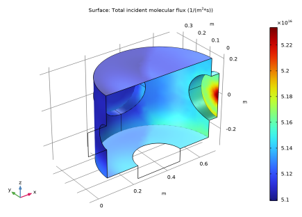
In the Model Builder window, expand the Results>Incident Molecular Flux (fmf) node, then click Surface.
2
In the Incident Molecular Flux (fmf) toolbar, click  Plot.
3
Click the  Zoom Extents button in the Graphics toolbar.
Compare the results with Figure 3.
Total Number Density (fmf)
1
In the Model Builder window, under Results click Total Number Density (fmf).
2
In the Total Number Density (fmf) toolbar, click  Plot.
3
Click the  Zoom Extents button in the Graphics toolbar.
Plot the mass flow rate as a function of the inverse Knudsen number.
Tube mass flow rate
1
In the Home toolbar, click  Add Plot Group and choose 1D Plot Group.
2
In the Settings window for 1D Plot Group, type Tube mass flow rate in the Label text field.
Global 1
1
Right-click Tube mass flow rate and choose Global.
2
In the Settings window for Global, locate the y-Axis Data section.
3
4
Click to expand the Legends section. Clear the Show legends check box.
5
Locate the x-Axis Data section. From the Parameter list, choose Expression.
6
In the Expression text field, type 1/Knm.
7
Click to expand the Coloring and Style section. Find the Line markers subsection. From the Marker list, choose Circle.
8
Click the  x-Axis Log Scale button in the Graphics toolbar.
9
Click the  y-Axis Log Scale button in the Graphics toolbar.
10
In the Tube mass flow rate toolbar, click  Plot.
Plot the normalized mass flow rate in the tube in order to see Knudsen’s minimum.
1D Plot Group 4
1
In the Home toolbar, click  Add Plot Group and choose 1D Plot Group.
2
In the Settings window for 1D Plot Group, locate the Legend section.
3
From the Position list, choose Upper left.
4
Locate the Plot Settings section.
5
Select the y-axis label check box. In the associated text field, type Normalized Flow Rate (1).
Global 1
1
Right-click 1D Plot Group 4 and choose Global.
2
In the Settings window for Global, locate the y-Axis Data section.
3
4
Locate the x-Axis Data section. From the Parameter list, choose Expression.
5
In the Expression text field, type 1/Knm.
6
Click the  x-Axis Log Scale button in the Graphics toolbar.
7
Click the  y-Axis Log Scale button in the Graphics toolbar.
8
Locate the Coloring and Style section. Find the Line markers subsection. From the Marker list, choose Diamond.
Normalized mass flow rate
1
In the Model Builder window, under Results click 1D Plot Group 4.
2
In the Settings window for 1D Plot Group, type Normalized mass flow rate in the Label text field.
3
In the Normalized mass flow rate toolbar, click  Plot.
Check the Knudsen number on the high vacuum side is in the free molecular flow regime.
Global Evaluation 1
1
In the Results toolbar, click  Global Evaluation.
2
In the Settings window for Global Evaluation, locate the Expressions section.
3
4
Click  Evaluate.
Table
1
Go to the Table window.
The lowest Knudsen number for the outlet is 5. At this low number there is some intramolecular scattering in the flow, but it is very limited. All the other results have Knudsen numbers greater than 10, so the free molecular flow assumption is justified.
Add a second instance of the Free Molecular Flow interface for comparison with the results obtained at low pressures when the flow in the entire tube is free molecular.
Add Physics
1
In the Home toolbar, click  Add Physics to open the Add Physics window.
2
Go to the Add Physics window.
3
In the tree, select Fluid Flow>Rarefied Flow>Free Molecular Flow (fmf).
4
Find the Physics interfaces in study subsection. In the table, clear the Solve check box for Study 1.
5
Click Add to Component 1 in the window toolbar.
6
In the Home toolbar, click  Add Physics to close the Add Physics window.
Add Study
1
In the Home toolbar, click  Add Study to open the Add Study window.
2
Go to the Add Study window.
3
Find the Studies subsection. In the Select Study tree, select General Studies>Stationary.
4
Click Add Study in the window toolbar.
5
In the Home toolbar, click  Add Study to close the Add Study window.
Free Molecular Flow 2 (fmf2)
1
In the Model Builder window, under Component 1 (comp1) click Free Molecular Flow 2 (fmf2).
2
Select the tube in addition to the high vacuum chamber.
3
In the Settings window for Free Molecular Flow, locate the Compute section.
4
Clear the Pressure check box.
5
Locate the Integration Settings section. From the Integration resolution list, choose 2048.
Molecular Flow 1
1
In the Model Builder window, under Component 1 (comp1)>Free Molecular Flow 2 (fmf2) click Molecular Flow 1.
2
In the Settings window for Molecular Flow, locate the Molecular Weight of Species section.
3
In the Mn,G2 text field, type Mn0.
Surface Temperature 1
1
In the Model Builder window, click Surface Temperature 1.
2
In the Settings window for Surface Temperature, locate the Surface Temperature section.
3
In the T text field, type T0.
Add the Vacuum Pump boundary condition. Divide the pump speed by two in order to account for the plane symmetry condition.
Vacuum Pump 1
1
In the Physics toolbar, click  Boundaries and choose Vacuum Pump.
2
In the Settings window for Vacuum Pump, locate the Boundary Selection section.
3
From the Selection list, choose Pump.
4
Locate the Vacuum Pump section. From the Specify pump flux list, choose Pump speed.
5
In the SG2 text field, type Spump/2.
The Reservoir boundary condition is used to represent the low vacuum part of the system.
Reservoir 1
1
In the Physics toolbar, click  Boundaries and choose Reservoir.
2
In the Settings window for Reservoir, locate the Boundary Selection section.
3
From the Selection list, choose Inlet.
4
Locate the Reservoir section. In the p0,G2 text field, type pa_inf.
Definitions
Define a nonlocal integration coupling at the inlet boundary to compute the total mass flow through the inlet.
Integration 1 (intop1)
1
In the Definitions toolbar, click  Nonlocal Couplings and choose Integration.
2
In the Settings window for Integration, locate the Source Selection section.
3
From the Geometric entity level list, choose Boundary.
4
From the Selection list, choose Inlet.
Add a second integration to check the mass flow out of the pump.
Integration 2 (intop2)
1
Right-click Integration 1 (intop1) and choose Duplicate.
2
In the Settings window for Integration, locate the Source Selection section.
3
Click  Clear Selection.
4
From the Selection list, choose Pump.
Free Molecular Flow 2 (fmf2)
Symmetry 1
1
In the Physics toolbar, click  Global and choose Symmetry.
2
Component 1 (comp1)
Create a new mesh that includes the tube.
Mesh 2
In the Mesh toolbar, click Add Mesh and choose Add Mesh.
Size 1
1
Right-click Mesh 2 and choose Size.
2
In the Settings window for Size, locate the Geometric Entity Selection section.
3
From the Geometric entity level list, choose Boundary.
4
From the Selection list, choose Port.
5
Locate the Element Size section. From the Calibrate for list, choose Fluid dynamics.
6
From the Predefined list, choose Extra fine.
This setting refines the mesh on the port opposite the outlet to better capture the molecular beaming from the tube.
Size
1
In the Model Builder window, click Size.
2
In the Settings window for Size, locate the Element Size section.
3
From the Predefined list, choose Extra fine.
Size 2
1
In the Model Builder window, right-click Mesh 2 and choose Size.
2
In the Settings window for Size, locate the Geometric Entity Selection section.
3
From the Geometric entity level list, choose Boundary.
4
From the Selection list, choose Inlet.
5
Locate the Element Size section. From the Calibrate for list, choose Fluid dynamics.
6
From the Predefined list, choose Extremely fine.
Free Triangular 1
1
In the Mesh toolbar, click  Boundary and choose Free Triangular.
2
In the Settings window for Free Triangular, locate the Boundary Selection section.
3
From the Selection list, choose Inlet.
4
Click  Build Selected.
Mapped 1
1
In the Mesh toolbar, click  Boundary and choose Mapped.
2
In the Settings window for Mapped, locate the Boundary Selection section.
3
From the Selection list, choose Tube.
Distribution 1
1
Right-click Mapped 1 and choose Distribution.
2
In the Settings window for Distribution, locate the Distribution section.
3
In the Number of elements text field, type 80.
4
Free Triangular 2
1
In the Mesh toolbar, click  Boundary and choose Free Triangular.
2
In the Settings window for Free Triangular, locate the Boundary Selection section.
3
From the Selection list, choose Chamber.
Free Triangular 3
1
In the Mesh toolbar, click  Boundary and choose Free Triangular.
2
3
In the Settings window for Free Triangular, click  Build All.
In Study 2 only the Free Molecular Flow 2 physics interface should be solved for.
Study 2
Step 1: Stationary
1
In the Model Builder window, under Study 2 click Step 1: Stationary.
2
In the Settings window for Stationary, locate the Physics and Variables Selection section.
3
In the table, clear the Solve for check box for Free Molecular Flow (fmf).
Use mesh 2.
4
Click to expand the Mesh Selection section. In the table, enter the following settings:
5
In the Home toolbar, click  Compute.
Results
Study 2/Solution 2 (3) (sol2)
In the Model Builder window, under Results>Datasets right-click Study 2/Solution 2 (sol2) and choose Duplicate.
Selection
1
In the Results toolbar, click  Attributes and choose Selection.
2
In the Settings window for Selection, locate the Geometric Entity Selection section.
3
From the Geometric entity level list, choose Boundary.
4
From the Selection list, choose Postprocessing.
Surface
1
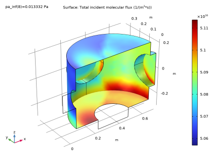
In the Model Builder window, expand the Results>Incident Molecular Flux (fmf2) node, then click Surface.
2
In the Incident Molecular Flux (fmf2) toolbar, click  Plot.
Compare the resulting plot with Figure 8.
Surface
1
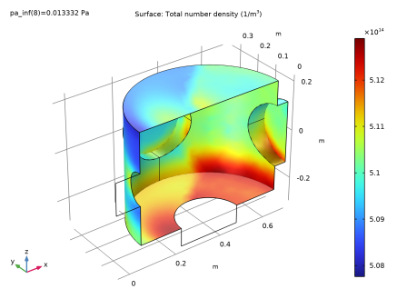
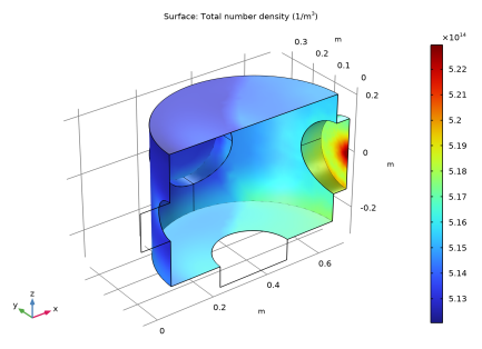
In the Model Builder window, expand the Results>Total Number Density (fmf2) node, then click Surface.
2
In the Total Number Density (fmf2) toolbar, click  Plot.
Compare the resulting plot with Figure 9.
Plot the number density along the tube.
Number density in the tube
1
In the Home toolbar, click  Add Plot Group and choose 1D Plot Group.
2
In the Settings window for 1D Plot Group, locate the Data section.
3
From the Dataset list, choose Study 2/Solution 2 (3) (sol2).
4
Locate the Plot Settings section.
5
Select the x-axis label check box. In the associated text field, type position (mm).
6
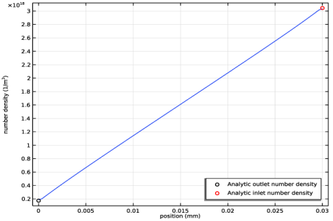
Select the y-axis label check box. In the associated text field, type number density (1/m<sup>3</sup>).
7
Locate the Legend section. From the Position list, choose Lower right.
8
Click to expand the Title section. From the Title type list, choose None.
9
In the Label text field, type Number density in the tube.
Line Graph 1
1
Right-click Number density in the tube and choose Line Graph.
2
3
In the Settings window for Line Graph, locate the y-Axis Data section.
4
In the Expression text field, type fmf2.ntot.
5
Locate the x-Axis Data section. From the Parameter list, choose Reversed arc length.
6
Click to expand the Quality section. From the Resolution list, choose No refinement.
Global 1
1
In the Model Builder window, right-click Number density in the tube and choose Global.
2
In the Settings window for Global, locate the y-Axis Data section.
3
4
Locate the x-Axis Data section. From the Parameter list, choose Expression.
5
In the Expression text field, type 0.
6
Locate the Coloring and Style section. Find the Line style subsection. From the Line list, choose None.
7
From the Color list, choose Black.
8
Find the Line markers subsection. From the Marker list, choose Circle.
9
Locate the y-Axis Data section. In the Description text field, type Analytic outlet number density.
Global 2
1
Right-click Number density in the tube and choose Global.
2
In the Settings window for Global, locate the y-Axis Data section.
3
4
In the Description text field, type Analytic inlet number density.
5
Locate the x-Axis Data section. From the Parameter list, choose Expression.
6
In the Expression text field, type 30[mm].
7
Locate the Coloring and Style section. Find the Line style subsection. From the Line list, choose None.
8
From the Color list, choose Red.
9
Find the Line markers subsection. From the Marker list, choose Circle.
Evaluate the mass flow into the system and compare with the analytic value and the flow out of the system. Multiply the nonlocal integration couplings by two in order to account for the plane symmetry condition.
Global Evaluation 2
1
In the Results toolbar, click  Global Evaluation.
2
In the Settings window for Global Evaluation, locate the Data section.
3
From the Dataset list, choose Study 2/Solution 2 (2) (sol2).
4
Locate the Expressions section. In the table, enter the following settings:
5
Click  Evaluate.
Global Evaluation 3
1
Right-click Global Evaluation 2 and choose Duplicate.
2
In the Settings window for Global Evaluation, locate the Expressions section.
3
4
Clicknext to  Evaluate, then choose Table 2 - Global Evaluation 2.
Global Evaluation 4
1
Right-click Global Evaluation 3 and choose Duplicate.
2
In the Settings window for Global Evaluation, locate the Expressions section.
3
4
Clicknext to  Evaluate, then choose Table 2 - Global Evaluation 2.
Table
1
Go to the Table window.
There is good agreement between the mass flow predicted by COMSOL and that produced by the analytic expressions. The mass conservation is also reasonable.
Appendix: Geometry Instructions
From the File menu, choose New.
New
In the New window, click  Blank Model.
Add Component
In the Home toolbar, click  Add Component and choose 3D.
Combining Cylinders
The geometry consists of several cylinders that are joined together.
Cylinder 1 (cyl1)
1
In the Geometry toolbar, click  Cylinder.
2
In the Settings window for Cylinder, locate the Size and Shape section.
3
In the Radius text field, type 0.3.
4
In the Height text field, type 0.45.
5
Locate the Position section. In the x text field, type 0.35.
6
In the z text field, type -0.225.
Cylinder 2 (cyl2)
1
In the Geometry toolbar, click  Cylinder.
2
In the Settings window for Cylinder, locate the Size and Shape section.
3
In the Radius text field, type 0.125.
4
In the Height text field, type 0.7.
5
Locate the Position section. In the x text field, type 0.35.
6
In the y text field, type -0.35.
7
Locate the Axis section. From the Axis type list, choose y-axis. By changing the axis, the cylinder is oriented accordingly.
Cylinder 3 (cyl3)
1
In the Geometry toolbar, click  Cylinder.
2
In the Settings window for Cylinder, locate the Size and Shape section.
3
In the Radius text field, type 0.125.
4
In the Height text field, type 0.075.
5
Locate the Position section. In the x text field, type 0.35.
6
In the z text field, type -0.3.
Cylinder 4 (cyl4)
1
In the Geometry toolbar, click  Cylinder.
2
In the Settings window for Cylinder, locate the Size and Shape section.
3
In the Radius text field, type 0.065.
4
In the Height text field, type 0.4.
5
Locate the Position section. In the x text field, type -0.05.
6
Locate the Axis section. From the Axis type list, choose x-axis.
Cylinder 5 (cyl5)
1
In the Geometry toolbar, click  Cylinder.
2
In the Settings window for Cylinder, locate the Size and Shape section.
3
In the Radius text field, type 0.125.
4
In the Height text field, type 0.35.
5
Locate the Position section. In the x text field, type 0.35.
6
Locate the Axis section. From the Axis type list, choose x-axis.
Union 1 (uni1)
1
In the Geometry toolbar, click  Booleans and Partitions and choose Union.
2
Click the  Select All button in the Graphics toolbar.
3
In the Settings window for Union, locate the Union section.
4
Clear the Keep interior boundaries check box. This combines the selected cylinders into an object with a single domain.
Cylinder 6 (cyl6)
1
In the Geometry toolbar, click  Cylinder.
2
In the Settings window for Cylinder, locate the Size and Shape section.
3
In the Radius text field, type 0.065.
4
In the Height text field, type 0.04.
5
Locate the Position section. In the x text field, type -0.1.
6
Locate the Axis section. From the Axis type list, choose x-axis.
Cone 1 (cone1)
1
In the Geometry toolbar, click  Cone.
2
In the Settings window for Cone, locate the Size and Shape section.
3
In the Bottom radius text field, type 20[mm].
4
In the Height text field, type 27[mm].
5
In the Top radius text field, type 15.5[mm].
6
Locate the Position section. In the x text field, type -0.08.
7
In the z text field, type -0.09.
Union 2 (uni2)
1
In the Geometry toolbar, click  Booleans and Partitions and choose Union.
2
Select the objects cone1 and cyl6 only.
3
In the Settings window for Union, locate the Union section.
4
Clear the Keep interior boundaries check box.
Cylinder 7 (cyl7)
1
In the Geometry toolbar, click  Cylinder.
2
In the Settings window for Cylinder, locate the Size and Shape section.
3
In the Radius text field, type 0.015.
4
In the Height text field, type 0.02.
5
Locate the Position section. In the x text field, type -0.08.
6
Locate the Axis section. From the Axis type list, choose x-axis.
Difference 1 (dif1)
1
In the Geometry toolbar, click  Booleans and Partitions and choose Difference.
2
3
In the Settings window for Difference, locate the Difference section.
4
Find the Objects to subtract subsection. Click to select the  Activate Selection toggle button.
5
Cylinder 8 (cyl8)
1
In the Geometry toolbar, click  Cylinder.
2
In the Settings window for Cylinder, locate the Size and Shape section.
3
In the Radius text field, type 1.5[mm].
4
In the Height text field, type 0.03.
5
Locate the Position section. In the x text field, type -0.08.
6
Locate the Axis section. From the Axis type list, choose x-axis.
Using Symmetry
The geometry and the physics are symmetrical with respect to the zx-plane. The geometry can therefore be partitioned to save mesh elements and computation resources.
Work Plane 1 (wp1)
1
In the Geometry toolbar, click  Work Plane.
2
In the Settings window for Work Plane, locate the Plane Definition section.
3
From the Plane list, choose zx-plane.
Partition Objects 1 (par1)
1
In the Geometry toolbar, click  Booleans and Partitions and choose Partition Objects.
2
Click in the Graphics window and then press Ctrl+A to select all objects.
3
In the Settings window for Partition Objects, locate the Partition Objects section.
4
From the Partition with list, choose Work plane.
Delete Entities 1 (del1)
1
In the Model Builder window, right-click Geometry 1 and choose Delete Entities.
2
In the Settings window for Delete Entities, locate the Entities or Objects to Delete section.
3
From the Geometric entity level list, choose Domain.
4
Select all Domains in the y half of the geometry.
5
On the object par1(1), select Domain 1 only.
6
On the object par1(2), select Domain 1 only.
7
On the object par1(3), select Domain 1 only.
8
Click  Build Selected.
Form Union (fin)
1
In the Model Builder window, click Form Union (fin).
2
In the Settings window for Form Union/Assembly, click  Build Selected.
Add Named Selections to the Geometry
Chamber Domain
1
In the Geometry toolbar, click  Selections and choose Explicit Selection.
2
In the Settings window for Explicit Selection, type Chamber Domain in the Label text field.
3
On the object fin, select Domain 3 only.
Chamber and Outlet
1
In the Geometry toolbar, click  Selections and choose Adjacent Selection.
2
In the Settings window for Adjacent Selection, type Chamber and Outlet in the Label text field.
3
Locate the Input Entities section. Click  Add.
4
In the Add dialog box, select Chamber Domain in the Input selections list.
5
Outlet
1
In the Geometry toolbar, click  Selections and choose Explicit Selection.
2
In the Settings window for Explicit Selection, type Outlet in the Label text field.
3
Locate the Entities to Select section. From the Geometric entity level list, choose Boundary.
4
Click the  Wireframe Rendering button in the Graphics toolbar.
5
On the object fin, select Boundary 19 only.
Chamber
1
In the Geometry toolbar, click  Selections and choose Difference Selection.
2
In the Settings window for Difference Selection, type Chamber in the Label text field.
3
Locate the Geometric Entity Level section. From the Level list, choose Boundary.
4
Locate the Input Entities section. Click  Add.
5
In the Add dialog box, select Chamber and Outlet in the Selections to add list.
6
7
In the Settings window for Difference Selection, locate the Input Entities section.
8
9
In the Add dialog box, select Outlet in the Selections to subtract list.
10
Inlet
1
In the Geometry toolbar, click  Selections and choose Explicit Selection.
2
In the Settings window for Explicit Selection, type Inlet in the Label text field.
3
Locate the Entities to Select section. From the Geometric entity level list, choose Boundary.
4
On the object fin, select Boundary 9 only.
Tube
1
In the Geometry toolbar, click  Selections and choose Explicit Selection.
2
In the Settings window for Explicit Selection, type Tube in the Label text field.
3
Locate the Entities to Select section. From the Geometric entity level list, choose Boundary.
4
Select the Group by continuous tangent check box.
5
On the object fin, select Boundaries 11 and 12 only.
Pump
1
In the Geometry toolbar, click  Selections and choose Explicit Selection.
2
In the Settings window for Explicit Selection, type Pump in the Label text field.
3
Locate the Entities to Select section. From the Geometric entity level list, choose Boundary.
4
On the object fin, select Boundary 25 only.
Port
1
In the Geometry toolbar, click  Selections and choose Explicit Selection.
2
In the Settings window for Explicit Selection, type Port in the Label text field.
3
Locate the Entities to Select section. From the Geometric entity level list, choose Boundary.
4
On the object fin, select Boundary 35 only.
Box Selection 1 (boxsel1)
1
In the Geometry toolbar, click  Selections and choose Box Selection.
2
In the Settings window for Box Selection, locate the Geometric Entity Level section.
3
From the Level list, choose Boundary.
4
Locate the Box Limits section. In the y minimum text field, type -0.1[mm].
5
Locate the Output Entities section. From the Include entity if list, choose Entity inside box.
Cylinder Selection 1 (cylsel1)
1
In the Geometry toolbar, click  Selections and choose Cylinder Selection.
2
In the Settings window for Cylinder Selection, locate the Size and Shape section.
3
In the Outer radius text field, type 0.1.
4
Locate the Axis section. From the Axis type list, choose x-axis.
5
Locate the Output Entities section. From the Include entity if list, choose Entity inside cylinder.
6
Locate the Geometric Entity Level section. From the Level list, choose Boundary.
Cylinder Selection 2 (cylsel2)
1
In the Geometry toolbar, click  Selections and choose Cylinder Selection.
2
In the Settings window for Cylinder Selection, locate the Geometric Entity Level section.
3
From the Level list, choose Boundary.
4
Locate the Size and Shape section. In the Outer radius text field, type 0.2.
5
Locate the Position section. In the x text field, type 0.35.
6
Locate the Output Entities section. From the Include entity if list, choose Entity inside cylinder.
Postprocessing
1
In the Geometry toolbar, click  Selections and choose Difference Selection.
2
In the Settings window for Difference Selection, type Postprocessing in the Label text field.
3
Locate the Geometric Entity Level section. From the Level list, choose Boundary.
4
Locate the Input Entities section. Click  Add.
5
In the Add dialog box, select Box Selection 1 in the Selections to add list.
6
7
In the Settings window for Difference Selection, locate the Input Entities section.
8
9
In the Add dialog box, in the Selections to subtract list, choose Cylinder Selection 1 and Cylinder Selection 2.
10