You are viewing the documentation for an older COMSOL version. The latest version is available here.
PDF

Three-Phase Mixer
Introduction
This example of a turbulent fluid-solid mixture in a mixer shows how to set up a time-dependent, turbulent three-phase flow simulation together with a rotating domain. The mixture is a suspension of a fluid and two particle populations, one population consisting of particles lighter than the fluid and the other of particles heavier than the fluid. Before the impeller starts to rotate, the mixture tends to separate since the light particles rise to the top of the tank and the heavy particles sediment at the bottom. When the suspension is stirred, the fluid and the particles mix again.
Model Definition
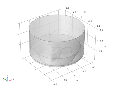
The mixer is an under-baffled stirred vessel. Figure 1 shows the model geometry. The tank is cylindrical with a three-bladed impeller placed close to the curved bottom. It has a diameter of 450 mm and a height of 300 mm. The tank is completely filled with the fluid-solid mixture and initially the distribution of both particle populations is homogeneous, with a volume fraction of 0.1.
Figure 1: Geometry of the mixer with a three-bladed impeller.
The suspension consists of water (with density and viscosity taken from the Water, liquid material from COMSOL’s built-in material library) and two particle populations with particle densities 1100 kg/m3 and 850 kg/m3, respectively. The particles in both populations have a diameter of 1 mm. The Hadamard–Rybczynski model is used to compute particle slip velocities, and the mixture viscosity is calculated using the Krieger model. The model uses a time-dependent simulation starting from rest. The impeller starts to rotate after 1.5 s and then the rotational velocity of the impeller is gradually increased until it reaches 100 rpm at t =2. 5 s. The simulation is continued until t = 10 s. The flow in the mixer is modeled using the Phase Transport Mixture Model Turbulent Flow, k-ε interface.
Results and Discussion
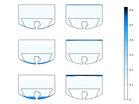
The results presented in this section concern the velocity of the mixture and the volume fractions of the two particle populations. During the initial 1.5 s, when the suspension is not stirred, the mixture separates, which is seen in Figure 2. The left column shows plots of the volume fraction of the heavy particles in the xz-cut plane at t = 0.5 s, t = 1 s, and t = 1.5 s. The heavy particles sediment at the bottom of the tank due to gravity. The right column shows the volume fraction of the light particles at the same time instances, and they accumulate at the top of the tank due to buoyancy forces.
Figure 2: Volume fractions of the heavy (left column) and light particles (right column) at t = 0.5 s, t = 1 s, and t = 1.5 s, (top to bottom rows).
At t = 1.5 s the impeller starts rotating and at t = 2.5 s it is rotating full speed at 100 rpm. Figure 3 and Figure 4 show arrow and slice plots of the velocity (magnitude) at t = 4 s and t = 10 s, respectively. The plots show that, even though the impeller has been rotating at full speed for 1.5 s, at t = 4 s the fluid near the top of the tank is still accelerating, since it has not yet reached its final rotational velocity, which is shown in Figure 4.
Figure 3: Velocity field at t = 4 s. The impeller is rotating at 100 rpm, but the rotation has not yet accelerated the fluid at the top of the tank to maximum speed.
Figure 5 through Figure 8 show slice plots of the volume fractions of both particle populations at t = 3 s, t = 5 s, t = 7 s, and t = 9 s to illustrate the progressive mixing: at t = 3 s, the heavy (blue gradient color scale) and the light (red gradient color scale) particles are still accumulated, respectively, at the bottom and top of the tank, while for later time instances the particles are more evenly spread. The plot for t = 9 s (Figure 8) shows that the particle distribution is still not completely homogeneous after 6.5 s of stirring at full speed. To obtain a more homogeneous distribution, a faster impeller speed is needed.
Figure 4: Velocity field at t = 10 s.
Figure 5: Volume fractions of the light particles (red gradient color scale) and heavy particles (blue gradient color scale) at t = 3 s.
Figure 6: Volume fractions of the light particles (red gradient color scale) and heavy particles (blue gradient color scale) at t = 5 s.
Figure 7: Volume fractions of the light particles (red gradient color scale) and heavy particles (blue gradient color scale) at t = 7 s.
Figure 8: Volume fractions of the light particles (red gradient color scale) and heavy particles (blue gradient color scale) at t = 9 s.
Application Library path: Mixer_Module/Tutorials/three_phase_mixer
Modeling Instructions
From the File menu, choose New.
New
In the New window, click  Model Wizard.
Model Wizard
1
In the Model Wizard window, click  3D.
2
In the Select Physics tree, select Fluid Flow>Multiphase Flow>Rotating Machinery, Phase Transport Mixture Model>Turbulent Flow>Turbulent Flow, k-ε.
3
Click Add.
4
Click  Study.
5
In the Select Study tree, select General Studies>Time Dependent.
6
Geometry 1
Import 1 (imp1)
1
In the Home toolbar, click  Import.
2
In the Settings window for Import, locate the Import section.
3
Click  Browse.
4
Form Union (fin)
1
In the Model Builder window, under Component 1 (comp1)>Geometry 1 click Form Union (fin).
2
In the Settings window for Form Union/Assembly, locate the Form Union/Assembly section.
3
From the Action list, choose Form an assembly.
Definitions
Ramp 1 (rm1)
1
In the Home toolbar, click  Functions and choose Local>Ramp.
2
In the Settings window for Ramp, locate the Parameters section.
3
In the Location text field, type 1.55.
4
Select the Cutoff check box.
5
Click to expand the Smoothing section. Select the Size of transition zone at start check box.
Materials
In the Home toolbar, click  Windows and choose Add Material from Library.
Add Material
1
Go to the Add Material window.
2
In the tree, select Built-in>Water, liquid.
3
Click Add to Component in the window toolbar.
Moving Mesh
Rotating Domain 1
1
In the Model Builder window, under Component 1 (comp1)>Moving Mesh click Rotating Domain 1.
2
3
In the Settings window for Rotating Domain, locate the Rotation section.
4
In the f text field, type 100[rpm]*rm1(t*1[1/s]).
Turbulent Flow, k-ε (spf)
1
In the Model Builder window, under Component 1 (comp1) click Turbulent Flow, k-ε (spf).
2
In the Settings window for Turbulent Flow, k-ε, locate the Physical Model section.
3
Select the Include gravity check box.
Wall 2
1
In the Physics toolbar, click  Boundaries and choose Wall.
2
3
In the Settings window for Wall, click to expand the Wall Movement section.
4
From the Translational velocity list, choose Zero (Fixed wall).
The Translational velocity is set to Zero (Fixed Wall) to ensure that the wall is not moving. If Automatic from frame is selected, the wall will rotate due to the angular velocity of the Rotating Domain.
Pressure Point Constraint 1
1
In the Physics toolbar, click  Points and choose Pressure Point Constraint.
2
Phase Transport (phtr)
1
In the Model Builder window, under Component 1 (comp1) click Phase Transport (phtr).
2
In the Settings window for Phase Transport, click to expand the Dependent Variables section.
3
Click  Add Volume Fraction.
Initial Values 1
1
In the Model Builder window, under Component 1 (comp1)>Phase Transport (phtr) click Initial Values 1.
2
In the Settings window for Initial Values, locate the Initial Values section.
3
In the s0,s2 text field, type 0.1.
4
In the s0,s3 text field, type 0.1.
Multiphysics
Mixture Model 1 (mfmm1)
1
In the Model Builder window, under Component 1 (comp1)>Multiphysics click Mixture Model 1 (mfmm1).
2
In the Settings window for Mixture Model, locate the Physical Model section.
3
In the μ text field, type mfmm1.muc*max(1-max(0,min(s2+s3,0.999*0.62))/0.62,eps)^(-2.5*0.62).
4
From the Slip model list, choose Hadamard-Rybczynski.
5
Locate the Dispersed Phase 2 Properties section. From the ρs2 list, choose User defined. In the associated text field, type 1100[kg/m^3].
6
Locate the Dispersed Phase 3 Properties section. From the ρs3 list, choose User defined. In the associated text field, type 850[kg/m^3].
Mesh 1
1
In the Model Builder window, under Component 1 (comp1) click Mesh 1.
2
In the Settings window for Mesh, locate the Physics-Controlled Mesh section.
3
From the Element size list, choose Coarser.
Study 1
Step 1: Time Dependent
1
In the Model Builder window, under Study 1 click Step 1: Time Dependent.
2
In the Settings window for Time Dependent, locate the Study Settings section.
3
In the Output times text field, type range(0,0.5,10).
Solution 1 (sol1)
1
In the Study toolbar, click  Show Default Solver.
2
In the Model Builder window, expand the Solution 1 (sol1) node.
3
In the Model Builder window, under Study 1>Solver Configurations>Solution 1 (sol1) click Time-Dependent Solver 1.
4
In the Settings window for Time-Dependent Solver, click to expand the Time Stepping section.
5
From the Steps taken by solver list, choose Strict.
6
In the Model Builder window, expand the Study 1>Solver Configurations>Solution 1 (sol1)>Time-Dependent Solver 1>Segregated 1 node, then click Velocity u, Pressure p.
7
In the Settings window for Segregated Step, click to expand the Method and Termination section.
8
From the Jacobian update list, choose On every iteration.
9
In the Model Builder window, under Study 1>Solver Configurations>Solution 1 (sol1)>Time-Dependent Solver 1>Segregated 1 click Volume fractions.
10
In the Settings window for Segregated Step, locate the Method and Termination section.
11
From the Jacobian update list, choose On every iteration.
12
Click  Compute.
Results
Cut Plane 1
1
In the Results toolbar, click  Cut Plane.
2
In the Settings window for Cut Plane, locate the Plane Data section.
3
From the Plane list, choose xz-planes.
2D Plot Group 6
1
In the Results toolbar, click  2D Plot Group.
2
In the Settings window for 2D Plot Group, locate the Data section.
3
From the Dataset list, choose Cut Plane 1.
Surface 1
1
Right-click 2D Plot Group 6 and choose Surface.
2
In the Settings window for Surface, locate the Expression section.
3
In the Expression text field, type s2.
4
Click to expand the Range section. Select the Manual color range check box.
5
In the Maximum text field, type 0.62.
6
Locate the Coloring and Style section. Click  Change Color Table.
7
In the Color Table dialog box, select Aurora>JupiterAuroraBorealis in the tree.
8
9
In the Settings window for Surface, locate the Coloring and Style section.
10
From the Color table transformation list, choose Reverse.
2D Plot Group 6
1
In the Model Builder window, click 2D Plot Group 6.
2
In the Settings window for 2D Plot Group, click to expand the Plot Array section.
3
Select the Enable check box.
4
From the Array shape list, choose Square.
5
From the Order list, choose Column-major.
6
Locate the Data section. From the Time (s) list, choose 1.5.
Surface 2
1
In the Model Builder window, under Results>2D Plot Group 6 right-click Surface 1 and choose Duplicate.
2
In the Settings window for Surface, locate the Data section.
3
From the Dataset list, choose Cut Plane 1.
4
From the Time (s) list, choose 1.
5
Click to expand the Inherit Style section. From the Plot list, choose Surface 1.
Surface 3
1
Right-click Surface 2 and choose Duplicate.
2
In the Settings window for Surface, locate the Data section.
3
From the Time (s) list, choose 0.5.
Surface 4
1
In the Model Builder window, under Results>2D Plot Group 6 right-click Surface 1 and choose Duplicate.
2
In the Settings window for Surface, locate the Expression section.
3
In the Expression text field, type s3.
4
Locate the Inherit Style section. From the Plot list, choose Surface 1.
Surface 5
1
Right-click Surface 4 and choose Duplicate.
2
In the Settings window for Surface, locate the Data section.
3
From the Dataset list, choose Cut Plane 1.
4
From the Time (s) list, choose 1.
Surface 6
1
Right-click Surface 5 and choose Duplicate.
2
In the Settings window for Surface, locate the Data section.
3
From the Time (s) list, choose 0.5.
2D Plot Group 6
1
Click the  Show Grid button in the Graphics toolbar.
2
In the Model Builder window, click 2D Plot Group 6.
3
In the Settings window for 2D Plot Group, click to expand the Title section.
4
From the Title type list, choose None.
5
Click the  Zoom Extents button in the Graphics toolbar.
The previous instructions created the plots of the volume fractions as shown in Figure 2.
The following instructions create the plots in Figure 3 and Figure 4.
Slice
1
In the Model Builder window, expand the Velocity (spf) node, then click Slice.
2
In the Settings window for Slice, locate the Plane Data section.
3
From the Plane list, choose xy-planes.
4
In the Planes text field, type 3.
5
Select the Interactive check box.
6
In the Shift text field, type 0.03.
Arrow Volume 1
1
In the Model Builder window, right-click Velocity (spf) and choose Arrow Volume.
2
In the Settings window for Arrow Volume, locate the Arrow Positioning section.
3
Find the x grid points subsection. In the Points text field, type 10.
4
Find the y grid points subsection. In the Points text field, type 10.
5
Find the z grid points subsection. From the Entry method list, choose Coordinates.
6
In the Coordinates text field, type 0.08 0.18 0.28.
Surface 1
Right-click Velocity (spf) and choose Surface.
Selection 1
1
In the Model Builder window, right-click Surface 1 and choose Selection.
2
In the Settings window for Selection, locate the Selection section.
3
Click  Paste Selection.
4
In the Paste Selection dialog box, type 2, 3, 9-34 in the Selection text field.
5
Material Appearance 1
1
In the Model Builder window, right-click Surface 1 and choose Material Appearance.
2
In the Settings window for Material Appearance, locate the Appearance section.
3
From the Appearance list, choose Custom.
4
From the Material type list, choose Steel.
Velocity (spf)
1
In the Model Builder window, under Results click Velocity (spf).
2
In the Settings window for 3D Plot Group, locate the Data section.
3
From the Time (s) list, choose 4.
4
In the Velocity (spf) toolbar, click  Plot.
This reproduces the plot in Figure 3. Reproduce the plot in Figure 4 by choosing 10 from the Times (s) list.
The following last set of instructions creates the plots in Figure 5 to Figure 8.
Volume Fraction (phtr)
1
In the Model Builder window, expand the Results>Volume Fraction (phtr) node, then click Volume Fraction (phtr).
2
In the Settings window for 3D Plot Group, locate the Plot Settings section.
3
From the Frame list, choose Spatial  (x, y, z).
Slice
1
In the Model Builder window, click Slice.
2
In the Settings window for Slice, locate the Expression section.
3
In the Expression text field, type s2.
4
Locate the Plane Data section. In the Planes text field, type 1.
5
Locate the Coloring and Style section. From the Coloring list, choose Gradient.
6
From the Bottom color list, choose Blue.
7
From the Color table transformation list, choose Reverse.
8
Click to expand the Range section. Select the Manual color range check box.
9
In the Minimum text field, type 0.
10
In the Maximum text field, type 0.62.
Slice 2
1
Right-click Slice and choose Duplicate.
2
In the Settings window for Slice, locate the Expression section.
3
In the Expression text field, type s3.
4
Locate the Plane Data section. From the Plane list, choose zx-planes.
5
In the Planes text field, type 1.
6
Locate the Coloring and Style section. From the Bottom color list, choose Red.
Surface 2
In the Model Builder window, under Results>Velocity (spf) right-click Surface 1 and choose Duplicate.
Surface 2
Drag and drop Surface 2 below Volume Fraction (phtr)
Slice
 2.
Volume Fraction (phtr)
1
In the Model Builder window, click Volume Fraction (phtr).
2
In the Settings window for 3D Plot Group, locate the Data section.
3
From the Time (s) list, choose 3.
4
In the Volume Fraction (phtr) toolbar, click  Plot.
This reproduces the plot in Figure 5. To reproduce the remaining plots, choose different time instances from the Times (s) list.