You are viewing the documentation for an older COMSOL version. The latest version is available here.
PDF

Free Surface Mixer
Introduction
This example of turbulent flow in a partially baffled mixer shows how to set up The Rotating Machinery, Turbulent Flow interfaces from the Mixer Module with free surface and stationary free surface features. The mixed fluid is water, and the flow is modeled using the k-ε turbulence model. Both frozen-rotor and time-dependent simulations are performed and compared. The mixer geometry used in this model corresponds to the one used by J.-P. Torré and others (Ref. 1).
Model Definition
The mixer is a glass-lined, under-baffled stirred vessel. Figure 1 shows the model geometry. It includes a three-bladed impeller and two beavertail baffles supported at the top of the vessel. The tank bottom is curved, allowing the three-bladed impeller to be placed close to the bottom. The cylindrical part of the tank has a diameter of 450 mm, and the initial water level is 700 mm. The two contoured baffles hang from the top of the mixer, and their lower part is 256 mm above the bottom of the vessel.
Figure 1: Geometry of the mixer with two rods and a three-bladed impeller.
The fluid contained in the mixer, water, is mixed using an impeller with a rotational velocity of 100 rpm. The flow in the mixer is modeled using the k-ε turbulence model.
The model is solved in two steps. First, a Frozen Rotor study is used to reach a good initial solution for the time-dependent study without having to solve the transient startup of the problem. In order to converge this step, a parametric sweep is used to first solve the model with a lower Reynolds number by using a higher value of the dynamic viscosity, and then computed again with the actual dynamic viscosity of the fluid. Then, a Time Dependent study is solved for a period of 1.8 seconds. This corresponds to 3 revolutions of the impeller.
Free surface
The top boundary corresponds to the two-phase interface separating the modeled water from the external air. In the transient case, this is modeled using the free surface feature and a deforming domain. Assuming that the dynamic viscosity and density of the air are negligible compared to the corresponding values for the water, so that the velocity and viscous stresses of the air do not affect the flow in the vessel, the following condition is applied for the normal stress:
Here pext = 0 Pa is the pressure outside the free surface domain, and σ is the water/air surface tension coefficient. The kinematic free surface condition sets the mesh to follow the motion of the fluid in the normal direction to the surface:
The free surface feature is not available in the frozen rotor study since the deformation of the mesh cannot be tracked. In this case, the Stationary Free Surface feature can be used to approximate the deformation of the free surface from the pressure distribution on the boundary. This boundary condition applies a slip condition together with an external pressure. After computing the frozen rotor simulation, a Stationary Free Surface study step can be used to evaluate the free surface deformation ηFS from the pressure obtained in the frozen rotor study using a linearized free surface condition:
Here x = x0 represents the position of the undisturbed surface.
Results and Discussion
The resulting velocity and free surface deformation in the mixer for the frozen-rotor and time-dependent studies are shown in Figure 2 and Figure 3, respectively. The turbulent viscosities are depicted in Figure 4 and Figure 5. It can be observed that the velocity field and turbulent viscosity obtained in the frozen-rotor simulation agree well with the time-dependent results. The stationary free surface feature is also able to provide a good prediction of the vortex induced deformation that develops on the free surface. However, the time-dependent study also provides the transient evolution of the free surface deformation and its instabilities.
Figure 2: Velocity field and free surface position for the frozen rotor study.
Figure 3: Velocity field and free surface position at t = 1.8 s.
Figure 4: Turbulent viscosity for the frozen rotor case.
Figure 5: Turbulent viscosity at t = 1.8 s.
Figure 6 and Figure 7 show the velocity distribution in one vertical and five horizontal cross sections. The larger velocities are observed near the rotating blades, which induce a flow toward the walls. Upon reaching the wall, vertical high speed streaks form along the outer walls, and the fluid velocity decreases toward the top of the vessel. A swirl flow pattern can be observed at the upper part of the tank, resulting in a small central vortex adjacent to the free surface.
Figure 6: Velocity field in the middle xy-plane at t = 1.8 s.
Figure 7: Velocity field in 5 xz-planes.
Notes About the COMSOL Implementation
This model has a large number of degrees of freedom and requires an iterative solver for optimal performance. The Algebraic Multigrid Solver suggested per default is optimal for the Time Dependent study. A Geometric Multigrid Solver should be used in the frozen rotor study step since the Algebraic Multigrid Solver is not suited for the Stationary Free Surface feature.
Reference
1. J.-P. Torré et al., “An Experimental and Computational Study of the Vortex Shape in a Partially Baffled Agitated Vessel,” Chem. Eng. Sci., vol. 62, no. 7, pp. 1915–1926, 2007.
Application Library path: Mixer_Module/Tutorials/free_surface_mixer
Modeling Instructions
From the File menu, choose New.
New
In the New window, click  Model Wizard.
Model Wizard
1
In the Model Wizard window, click  3D.
2
In the Select Physics tree, select Fluid Flow>Single-Phase Flow>Rotating Machinery, Fluid Flow>Turbulent Flow>Turbulent Flow, k-ε.
3
Click Add.
4
Click  Study.
5
In the Select Study tree, select Preset Studies for Selected Physics Interfaces>Frozen Rotor with Stationary Free Surface.
6
Load the model geometry from a geometry sequence.
Geometry 1
1
In the Geometry toolbar, click  Insert Sequence.
2
3
In the Geometry toolbar, click  Build All.
Global Definitions
Parameters 1
1
In the Model Builder window, under Global Definitions click Parameters 1.
2
In the Settings window for Parameters, locate the Parameters section.
3
Step 1 (step1)
1
In the Home toolbar, click  Functions and choose Global>Step.
2
In the Settings window for Step, locate the Parameters section.
3
In the Location text field, type 0.5.
4
Click to expand the Smoothing section. From the Number of continuous derivatives list, choose 1.
5
Moving Mesh
Rotating Domain 1
1
In the Model Builder window, under Component 1 (comp1)>Moving Mesh click Rotating Domain 1.
2
3
In the Settings window for Rotating Domain, locate the Rotation section.
4
In the f text field, type 100[rpm].
5
Locate the Axis section. Specify the urot vector as
Component 1 (comp1)
Deforming Domain 1
1
In the Definitions toolbar, click  Moving Mesh and choose Domains>Deforming Domain.
2
Turbulent Flow, k-ε (spf)
1
In the Model Builder window, under Component 1 (comp1) click Turbulent Flow, k-ε (spf).
2
In the Settings window for Turbulent Flow, k-ε, locate the Physical Model section.
3
Select the Include gravity check box.
Gravity 1
1
In the Model Builder window, under Component 1 (comp1)>Turbulent Flow, k-ε (spf) click Gravity 1.
2
In the Settings window for Gravity, locate the Acceleration of Gravity section.
3
Specify the g vector as
Wall 2
1
In the Physics toolbar, click  Boundaries and choose Wall.
2
3
In the Settings window for Wall, click to expand the Wall Movement section.
4
From the Translational velocity list, choose Zero (Fixed wall).
The Translational velocity is set to Zero (Fixed Wall) to ensure that the wall is not moving. If Automatic from frame is selected, the wall will rotate due to the angular velocity of the Rotating Domain.
Stationary Free Surface 1
1
In the Physics toolbar, click  Boundaries and choose Stationary Free Surface.
2
Free Surface 1
1
In the Physics toolbar, click  Boundaries and choose Free Surface.
2
The Stationary Free Surface will be used in the Frozen Rotor study, while Free Surface will override it in the Time Dependent study.
Add Material
1
In the Home toolbar, click  Add Material to open the Add Material window.
2
Go to the Add Material window.
3
In the tree, select Built-in>Water, liquid.
4
Right-click and choose Add to Component 1 (comp1).
5
In the Home toolbar, click  Add Material to close the Add Material window.
Materials
Water, liquid (mat1)
1
In the Settings window for Material, locate the Material Contents section.
2
Mesh 1
Size
1
In the Model Builder window, under Component 1 (comp1) right-click Mesh 1 and choose Edit Physics-Induced Sequence.
2
In the Settings window for Size, locate the Element Size section.
3
Click the Custom button.
4
Locate the Element Size Parameters section. In the Maximum element size text field, type 0.02.
5
In the Minimum element size text field, type 0.008.
6
In the Maximum element growth rate text field, type 1.12.
Size 1
1
In the Model Builder window, click Size 1.
2
In the Settings window for Size, locate the Element Size section.
3
From the Predefined list, choose Fine.
4
Click the Custom button.
5
Locate the Element Size Parameters section.
6
Select the Maximum element size check box. In the associated text field, type 0.02.
7
Select the Minimum element size check box. In the associated text field, type 0.004.
8
Select the Maximum element growth rate check box. In the associated text field, type 1.12.
9
Select the Curvature factor check box.
10
Select the Resolution of narrow regions check box.
Free Tetrahedral 1
1
In the Model Builder window, click Free Tetrahedral 1.
2
In the Settings window for Free Tetrahedral, locate the Domain Selection section.
3
From the Geometric entity level list, choose Domain.
4
Size 1
1
Right-click Free Tetrahedral 1 and choose Size.
2
In the Settings window for Size, locate the Geometric Entity Selection section.
3
From the Geometric entity level list, choose Boundary.
4
Click  Paste Selection.
5
In the Paste Selection dialog box, type 2, 3, 5, 21, 30, 31, 32 in the Selection text field.
6
7
In the Settings window for Size, locate the Element Size section.
8
From the Predefined list, choose Extra fine.
9
Click the Custom button.
10
Locate the Element Size Parameters section.
11
Select the Maximum element size check box. In the associated text field, type 0.013.
12
Select the Curvature factor check box. In the associated text field, type 0.35.
Size 2
1
Right-click Free Tetrahedral 1 and choose Size.
2
In the Settings window for Size, locate the Geometric Entity Selection section.
3
From the Geometric entity level list, choose Boundary.
4
Click  Paste Selection.
5
In the Paste Selection dialog box, type 34, 38, 56 in the Selection text field.
6
7
In the Settings window for Size, locate the Element Size section.
8
From the Predefined list, choose Extremely fine.
Free Tetrahedral 1
Right-click Free Tetrahedral 1 and choose Build Selected.
Swept 1
1
In the Mesh toolbar, click  Swept.
2
In the Settings window for Swept, locate the Domain Selection section.
3
From the Geometric entity level list, choose Domain.
4
Distribution 1
1
Right-click Swept 1 and choose Distribution.
2
In the Settings window for Distribution, locate the Distribution section.
3
From the Distribution type list, choose Predefined.
4
In the Number of elements text field, type 16.
5
In the Element ratio text field, type 1.6.
Swept 2
In the Mesh toolbar, click  Swept.
Distribution 1
1
Right-click Swept 2 and choose Distribution.
2
In the Settings window for Distribution, locate the Distribution section.
3
From the Distribution type list, choose Predefined.
4
In the Number of elements text field, type 12.
5
In the Element ratio text field, type 2.
Boundary Layer Properties 1
1
In the Model Builder window, expand the Boundary Layers 1 node, then click Boundary Layer Properties 1.
2
In the Settings window for Boundary Layer Properties, locate the Layers section.
3
In the Number of layers text field, type 6.
4
In the Thickness adjustment factor text field, type 2.
5
Click  Build All.
6
Click the  Transparency button in the Graphics toolbar.
7
Click the  Transparency button in the Graphics toolbar.
Build manual multigrid levels for optimal performance.
Mesh 2
In the Mesh toolbar, click Add Mesh and choose Add Mesh.
Reference 1
1
In the Mesh toolbar, click  Modify and choose Reference.
2
In the Settings window for Reference, locate the Reference section.
3
From the Mesh list, choose Mesh 1.
Scale 1
1
In the Mesh toolbar, click  More Attributes and choose Scale.
2
In the Settings window for Scale, locate the Scale section.
3
In the Element size scale text field, type 2.
Reference 1
In the Model Builder window, right-click Reference 1 and choose Expand.
Size
1
In the Model Builder window, under Component 1 (comp1)>Meshes>Mesh 2 click Size.
2
In the Settings window for Size, locate the Element Size Parameters section.
3
In the Minimum element size text field, type 0.009*2.
Size 1
1
In the Model Builder window, click Size 1.
2
In the Settings window for Size, locate the Element Size Parameters section.
3
In the Minimum element size text field, type 0.004*2.
4
Click  Build All.
Mesh 3
In the Mesh toolbar, click Add Mesh and choose Add Mesh.
Reference 1
1
In the Mesh toolbar, click  Modify and choose Reference.
2
In the Settings window for Reference, locate the Reference section.
3
From the Mesh list, choose Mesh 2.
Scale 1
1
In the Mesh toolbar, click  More Attributes and choose Scale.
2
In the Settings window for Scale, locate the Scale section.
3
In the Element size scale text field, type 2.
Reference 1
In the Model Builder window, right-click Reference 1 and choose Expand.
Size 1
1
In the Model Builder window, under Component 1 (comp1)>Meshes>Mesh 3 click Size 1.
2
In the Settings window for Size, locate the Element Size Parameters section.
3
In the Minimum element size text field, type 0.004*4.
Size
1
In the Model Builder window, click Size.
2
In the Settings window for Size, locate the Element Size Parameters section.
3
In the Minimum element size text field, type 0.009*4.
4
Click  Build All.
Disable Deforming Domain in the frozen rotor study.
Study 1
Step 1: Frozen Rotor
1
In the Model Builder window, under Study 1 click Step 1: Frozen Rotor.
2
In the Settings window for Frozen Rotor, locate the Physics and Variables Selection section.
3
Select the Modify model configuration for study step check box.
4
In the tree, select Component 1 (comp1)>Moving Mesh, Controls spatial frame>Deforming Domain 1.
5
Click  Disable.
6
Click to expand the Mesh Selection section. In the table, enter the following settings:
7
Click to expand the Study Extensions section. Select the Auxiliary sweep check box.
8
9
10
From the Run continuation for list, choose No parameter.
11
From the Reuse solution from previous step list, choose Yes.
12
Click the  Show More Options button in the Model Builder toolbar.
13
In the Show More Options dialog box, in the tree, select the check box for the node Study>Multigrid Level.
14
15
Right-click Study 1>Step 1: Frozen Rotor and choose Multigrid Level.
16
In the Settings window for Multigrid Level, locate the Mesh Selection section.
17
18
In the Model Builder window, right-click Step 1: Frozen Rotor and choose Multigrid Level.
Step 2: Stationary Free Surface
1
In the Settings window for Stationary Free Surface, locate the Physics and Variables Selection section.
2
Select the Modify model configuration for study step check box.
3
In the tree, select Component 1 (comp1)>Moving Mesh, Controls spatial frame>Deforming Domain 1.
4
5
Click to expand the Mesh Selection section. In the table, enter the following settings:
Solution 1 (sol1)
1
In the Study toolbar, click  Show Default Solver.
2
In the Model Builder window, expand the Solution 1 (sol1) node.
3
In the Model Builder window, expand the Study 1>Solver Configurations>Solution 1 (sol1)>Stationary Solver 1>Segregated 1 node.
4
In the Model Builder window, expand the Study 1>Solver Configurations>Solution 1 (sol1)>Stationary Solver 1>AMG, fluid flow variables () node, then click Multigrid 1.
5
In the Settings window for Multigrid, locate the General section.
6
From the Hierarchy generation method list, choose Manual.
7
In the Study toolbar, click  Compute.
Before working with plots, disable the automatic update of plots. Due to the size of the datasets created, it is more convenient to generate plots actively.
Results
1
In the Model Builder window, click Results.
2
In the Settings window for Results, locate the Update of Results section.
3
Select the Only plot when requested check box.
Exterior Walls, Frozen Rotor
1
In the Model Builder window, expand the Results>Datasets node, then click Exterior Walls.
2
In the Settings window for Surface, type Exterior Walls, Frozen Rotor in the Label text field.
3
Locate the Selection section. In the list, choose 17 and 19.
4
Click  Remove from Selection.
5
Free Surface, Frozen Rotor
1
In the Results toolbar, click  More Datasets and choose Surface.
2
In the Settings window for Surface, type Free Surface, Frozen Rotor in the Label text field.
3
Velocity, Frozen Rotor
1
In the Model Builder window, under Results click Velocity (spf).
2
In the Settings window for 3D Plot Group, type Velocity, Frozen Rotor in the Label text field.
3
Locate the Plot Settings section. Clear the Plot dataset edges check box.
Slice
1
In the Model Builder window, expand the Velocity, Frozen Rotor node.
2
Right-click Results>Velocity, Frozen Rotor>Slice and choose Delete.
Surface 1
1
In the Model Builder window, right-click Velocity, Frozen Rotor and choose Surface.
2
In the Settings window for Surface, locate the Data section.
3
From the Dataset list, choose Free Surface, Frozen Rotor.
4
Locate the Coloring and Style section. Click  Change Color Table.
5
In the Color Table dialog box, select Wave>WaveLight in the tree.
6
Deformation 1
1
Right-click Surface 1 and choose Deformation.
2
In the Settings window for Deformation, locate the Expression section.
3
In the x component text field, type 0.
4
In the y component text field, type spf.etaFS.
5
In the z component text field, type 0.
6
Locate the Scale section. Select the Scale factor check box.
Arrow Volume 1
1
In the Model Builder window, right-click Velocity, Frozen Rotor and choose Arrow Volume.
2
In the Settings window for Arrow Volume, locate the Arrow Positioning section.
3
Find the x grid points subsection. In the Points text field, type 30.
4
Find the y grid points subsection. In the Points text field, type 3.
5
Find the z grid points subsection. In the Points text field, type 30.
6
Locate the Coloring and Style section.
7
Select the Scale factor check box. In the associated text field, type 0.07.
Color Expression 1
1
Right-click Arrow Volume 1 and choose Color Expression.
2
In the Settings window for Color Expression, locate the Coloring and Style section.
3
Click  Change Color Table.
4
In the Color Table dialog box, select Rainbow>RainbowLight in the tree.
5
Surface 2
1
In the Model Builder window, right-click Velocity, Frozen Rotor and choose Surface.
2
In the Settings window for Surface, locate the Data section.
3
From the Dataset list, choose Exterior Walls, Frozen Rotor.
4
Locate the Coloring and Style section. From the Coloring list, choose Uniform.
5
From the Color list, choose Gray.
6
In the Velocity, Frozen Rotor toolbar, click  Plot.
Pressure, Frozen Rotor
1
In the Model Builder window, under Results click Pressure (spf).
2
In the Settings window for 3D Plot Group, type Pressure, Frozen Rotor in the Label text field.
3
In the Pressure, Frozen Rotor toolbar, click  Plot.
Wall Resolution, Frozen Rotor
1
In the Model Builder window, under Results click Wall Resolution (spf).
2
In the Settings window for 3D Plot Group, type Wall Resolution, Frozen Rotor in the Label text field.
3
In the Wall Resolution, Frozen Rotor toolbar, click  Plot.
Turbulent Viscosity, Frozen Rotor
1
In the Home toolbar, click  Add Plot Group and choose 3D Plot Group.
2
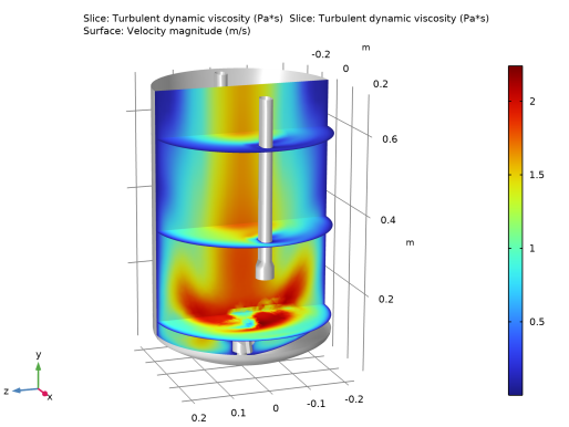
In the Settings window for 3D Plot Group, type Turbulent Viscosity, Frozen Rotor in the Label text field.
3
Locate the Plot Settings section. Clear the Plot dataset edges check box.
Slice 1
1
Right-click Turbulent Viscosity, Frozen Rotor and choose Slice.
2
In the Settings window for Slice, locate the Expression section.
3
In the Expression text field, type spf.muT.
4
Locate the Plane Data section. In the Planes text field, type 1.
Slice 2
1
Right-click Slice 1 and choose Duplicate.
2
In the Settings window for Slice, locate the Plane Data section.
3
From the Plane list, choose zx-planes.
4
In the Planes text field, type 3.
5
Click to expand the Inherit Style section. From the Plot list, choose Slice 1.
Surface 1
1
In the Model Builder window, right-click Turbulent Viscosity, Frozen Rotor and choose Surface.
2
In the Settings window for Surface, locate the Data section.
3
From the Dataset list, choose Exterior Walls, Frozen Rotor.
4
Locate the Coloring and Style section. From the Coloring list, choose Uniform.
5
From the Color list, choose Gray.
6
In the Turbulent Viscosity, Frozen Rotor toolbar, click  Plot.
Velocity xz, Frozen Rotor
1
In the Home toolbar, click  Add Plot Group and choose 3D Plot Group.
2
In the Settings window for 3D Plot Group, type Velocity xz, Frozen Rotor in the Label text field.
3
Locate the Plot Settings section. Clear the Plot dataset edges check box.
Slice 1
1
Right-click Velocity xz, Frozen Rotor and choose Slice.
2
In the Settings window for Slice, locate the Plane Data section.
3
From the Plane list, choose zx-planes.
4
In the Velocity xz, Frozen Rotor toolbar, click  Plot.
Add Study
1
In the Home toolbar, click  Add Study to open the Add Study window.
2
Go to the Add Study window.
3
Find the Studies subsection. In the Select Study tree, select General Studies>Time Dependent.
4
5
In the Home toolbar, click  Add Study to close the Add Study window.
Study 2
Step 1: Time Dependent
1
In the Settings window for Time Dependent, locate the Study Settings section.
2
In the Output times text field, type range(0,0.05,1.8).
3
Click to expand the Values of Dependent Variables section. Find the Initial values of variables solved for subsection. From the Settings list, choose User controlled.
4
From the Method list, choose Solution.
5
From the Study list, choose Study 1, Stationary Free Surface.
6
From the Selection list, choose Last.
7
Click to expand the Mesh Selection section. In the table, enter the following settings:
8
In the Study toolbar, click  Get Initial Value.
Results
Exterior Walls, Time Dependent
1
In the Model Builder window, under Results>Datasets click Exterior Walls.
2
In the Settings window for Surface, type Exterior Walls, Time Dependent in the Label text field.
3
Locate the Selection section. In the list, choose 17 and 19.
4
Click  Remove from Selection.
5
Free Surface, Time Dependent
1
In the Model Builder window, right-click Free Surface, Frozen Rotor and choose Duplicate.
2
In the Settings window for Surface, type Free Surface, Time Dependent in the Label text field.
3
Locate the Data section. From the Dataset list, choose Study 2/Solution 3 (sol3).
xy-Plane, Time Dependent
1
In the Results toolbar, click  Cut Plane.
2
In the Settings window for Cut Plane, type xy-Plane, Time Dependent in the Label text field.
3
Locate the Data section. From the Dataset list, choose Study 2/Solution 3 (sol3).
4
Locate the Plane Data section. From the Plane list, choose xy-planes.
Velocity, Time Dependent
1
In the Model Builder window, under Results click Velocity (spf).
2
In the Settings window for 3D Plot Group, type Velocity, Time Dependent in the Label text field.
3
Locate the Plot Settings section. Clear the Plot dataset edges check box.
Slice
1
In the Model Builder window, expand the Velocity, Time Dependent node.
2
Right-click Results>Velocity, Time Dependent>Slice and choose Delete.
Surface 1
1
In the Model Builder window, right-click Velocity, Time Dependent and choose Surface.
2
In the Settings window for Surface, locate the Data section.
3
From the Dataset list, choose Free Surface, Time Dependent.
4
Locate the Coloring and Style section. Click  Change Color Table.
5
In the Color Table dialog box, select Wave>WaveLight in the tree.
6
Arrow Volume 1
1
Right-click Velocity, Time Dependent and choose Arrow Volume.
2
In the Settings window for Arrow Volume, locate the Arrow Positioning section.
3
Find the x grid points subsection. In the Points text field, type 30.
4
Find the y grid points subsection. In the Points text field, type 3.
5
Find the z grid points subsection. In the Points text field, type 30.
6
Locate the Coloring and Style section.
7
Select the Scale factor check box. In the associated text field, type 0.07.
Color Expression 1
1
Right-click Arrow Volume 1 and choose Color Expression.
2
In the Settings window for Color Expression, locate the Coloring and Style section.
3
Click  Change Color Table.
4
In the Color Table dialog box, select Rainbow>RainbowLight in the tree.
5
Surface 2
1
In the Model Builder window, right-click Velocity, Time Dependent and choose Surface.
2
In the Settings window for Surface, locate the Data section.
3
From the Dataset list, choose Exterior Walls, Time Dependent.
4
Locate the Coloring and Style section. From the Coloring list, choose Uniform.
5
From the Color list, choose Gray.
Pressure, Time Dependent
1
In the Model Builder window, under Results click Pressure (spf).
2
In the Settings window for 3D Plot Group, type Pressure, Time Dependent in the Label text field.
Wall Resolution, Time Dependent
1
In the Model Builder window, under Results click Wall Resolution (spf).
2
In the Settings window for 3D Plot Group, type Wall Resolution, Time Dependent in the Label text field.
Study 2
Step 1: Time Dependent
1
In the Model Builder window, under Study 2 click Step 1: Time Dependent.
2
In the Settings window for Time Dependent, click to expand the Results While Solving section.
3
Select the Plot check box.
4
From the Plot group list, choose Velocity, Time Dependent.
Solver Configurations
In the Model Builder window, expand the Study 2>Solver Configurations node.
Solution 3 (sol3)
1
In the Model Builder window, expand the Study 2>Solver Configurations>Solution 3 (sol3) node.
2
In the Model Builder window, click Time-Dependent Solver 1.
3
In the Settings window for Time-Dependent Solver, click to expand the Time Stepping section.
4
From the Minimum BDF order list, choose 2.
The BDF order must be larger than one to accurately capture the surface movement.
5
Find the Algebraic variable settings subsection. In the Fraction of initial step for Backward Euler text field, type 1.
The initial time-step is already rather small, so the initialization time-step can be of the same order of magnitude. This will make the initialization easier.
6
In the Home toolbar, click  Compute.
Results
Velocity, Time Dependent
In the Velocity, Time Dependent toolbar, click  Plot.
Turbulent Viscosity, Time Dependent
1
In the Home toolbar, click  Add Plot Group and choose 3D Plot Group.
2
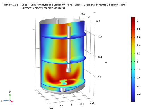
In the Settings window for 3D Plot Group, type Turbulent Viscosity, Time Dependent in the Label text field.
3
Locate the Data section. From the Dataset list, choose Study 2/Solution 3 (sol3).
4
Locate the Plot Settings section. Clear the Plot dataset edges check box.
Slice 1
1
Right-click Turbulent Viscosity, Time Dependent and choose Slice.
2
In the Settings window for Slice, locate the Expression section.
3
In the Expression text field, type spf.muT.
4
Locate the Plane Data section. In the Planes text field, type 1.
Slice 2
1
Right-click Slice 1 and choose Duplicate.
2
In the Settings window for Slice, locate the Plane Data section.
3
From the Plane list, choose zx-planes.
4
In the Planes text field, type 3.
5
Locate the Inherit Style section. From the Plot list, choose Slice 1.
Surface 1
1
In the Model Builder window, right-click Turbulent Viscosity, Time Dependent and choose Surface.
2
In the Settings window for Surface, locate the Data section.
3
From the Dataset list, choose Exterior Walls, Time Dependent.
4
Locate the Coloring and Style section. From the Coloring list, choose Uniform.
5
From the Color list, choose Gray.
6
In the Turbulent Viscosity, Time Dependent toolbar, click  Plot.
Velocity xy, Time Dependent
1
In the Home toolbar, click  Add Plot Group and choose 2D Plot Group.
2
In the Settings window for 2D Plot Group, type Velocity xy, Time Dependent in the Label text field.
3
Locate the Data section. From the Dataset list, choose xy-Plane, Time Dependent.
4
Locate the Plot Settings section. Clear the Plot dataset edges check box.
Surface 1
Right-click Velocity xy, Time Dependent and choose Surface.
Arrow Surface 1
1
In the Model Builder window, right-click Velocity xy, Time Dependent and choose Arrow Surface.
2
In the Settings window for Arrow Surface, locate the Arrow Positioning section.
3
Find the x grid points subsection. In the Points text field, type 20.
4
Find the y grid points subsection. In the Points text field, type 20.
5
Locate the Coloring and Style section.
6
Select the Scale factor check box. In the associated text field, type 0.1.
7
In the Velocity xy, Time Dependent toolbar, click  Plot.