You are viewing the documentation for an older COMSOL version. The latest version is available here.
PDF

Split and Recombine Mixer Benchmark
Introduction
Benchmarking is an important part of CFD research and code validation. This model uses COMSOL to compute multilamination by a split and recombine mixer. The flow pattern is visualized using a tracer and diffusion is suppressed by setting the diffusion coefficient to an extremely low value of 2·10–20 m2/s. Thus only numerical diffusion is significant in the model.
This model performs two separate stationary analyses, solving first for the flow and then for the convection/diffusion.
Model Definition
The geometry is constructed with two inlets and a single outlet to allow a flow of high concentration to mix with a flow of low concentration. The two flows primarily mix via multilamination as the flows get split and subsequently recombined as they proceed along the geometry.
Figure 1: Model geometry. The flow lamination pattern is studied at the cross sections indicated.
The model studies the flow lamination pattern at various places along the mixer channel, labeled A–A, B–B, C–C, and D–D in Figure 1.
Results and Discussion
Figure 2 shows the lamination patterns at the four locations. The blur on the interfaces is due to numerical diffusion within the simulation. High numerical diffusion would result in a more pronounced blurring of the interface. It is clear that the calculated interfaces are sharp indicating little numerical diffusion in the results. These flow patterns are in good agreement with those presented by Glatzel and others (Ref. 1).
Figure 2: Flow lamination patterns at locations A–A, B–B, C–C, and D–D.
The total pressure drop at a given flow rate (fluidic resistance) across the mixer is calculated to be 1.63 Pa. This result is slightly lower that obtained by the other codes in Ref. 1. However a lower value is expected as the finite-element method adds less artificial diffusion to the problem than the finite-volume method. Adding artificial diffusion to a flow problem increases the effective viscosity of the fluid and is therefore expected to artificially increase the pressure drop across the system.
Reference
1. T. Glatzel, C. Litterst, C. Cupelli, T. Lindemann, C. Moosmann, R. Niekrawietz, W. Streule, R. Zengerle, and P. Koltay, “Computational fluid dynamics (CFD) software tools for microfluidic applications - A case study,” Computers & Fluids, vol. 37, pp. 218–235, 2008.
Notes About the COMSOL Implementation
The model is straightforward to set up using a Laminar Flow interface together with a Transport of Diluted Species interface. The Transport in Diluted Species interface uses the solution from the Laminar Flow interface. This solution coupling is demonstrated in this model.
Application Library path: Microfluidics_Module/Micromixers/split_recombine_mixer
Modeling Instructions
From the File menu, choose New.
New
In the New window, click  Model Wizard.
Model Wizard
1
In the Model Wizard window, click  3D.
2
In the Select Physics tree, select Chemical Species Transport>Reacting Flow>Laminar Flow, Diluted Species.
3
Click Add.
4
Click  Study.
5
In the Select Study tree, select General Studies>Stationary.
6
Geometry 1
For convenience, the device geometry is inserted from an existing file. You can read the instructions for creating the geometry in the Appendix — Geometry Instructions.
1
In the Geometry toolbar, click Insert Sequence and choose Insert Sequence.
2
3
In the Geometry toolbar, click  Build All.
The geometry should look like that in Figure 1.
Materials
Fluid
1
In the Model Builder window, under Component 1 (comp1) right-click Materials and choose Blank Material.
2
In the Settings window for Material, type Fluid in the Label text field.
3
Locate the Material Contents section. In the table, enter the following settings:
Global Definitions
Parameters 1
1
In the Model Builder window, under Global Definitions click Parameters 1.
2
In the Settings window for Parameters, locate the Parameters section.
3
Laminar Flow (spf)
1
In the Model Builder window, under Component 1 (comp1) click Laminar Flow (spf).
2
In the Settings window for Laminar Flow, click to expand the Discretization section.
3
From the Discretization of fluids list, choose P2+P1.
Two inlets are defined to allow the introduction of the two fluid streams. One stream will carry the tracer.
Inlet 1
1
In the Physics toolbar, click  Boundaries and choose Inlet.
2
In the Settings window for Inlet, locate the Boundary Selection section.
3
From the Selection list, choose Inlet.
4
Locate the Velocity section. In the U0 text field, type v0.
Outlet 1
1
In the Physics toolbar, click  Boundaries and choose Outlet.
2
In the Settings window for Outlet, locate the Boundary Selection section.
3
From the Selection list, choose Outlet.
Transport of Diluted Species (tds)
Streamline and crosswind diffusion are activated by default. There are two options available for the type of crosswind diffusion used to provide numerical stabilization. The default option, Do Carmo and Galeao is more effective at suppressing undershoots and overshoots in the concentration, whereas the second option, Codina produces less artificial diffusion in the crosswind direction. Make the stabilization settings available following the steps below.
1
Click the  Show More Options button in the Model Builder toolbar.
2
In the Show More Options dialog box, in the tree, select the check box for the node Physics>Stabilization.
3
4
In the Model Builder window, under Component 1 (comp1) click Transport of Diluted Species (tds).
5
In the Settings window for Transport of Diluted Species, click to expand the Consistent Stabilization section.
6
From the Crosswind diffusion type list, choose Codina.
7
Click to expand the Discretization section. From the Concentration list, choose Cubic.
Choosing cubic discretization for the concentration reduces the numerical diffusion. To suppress physical diffusion, set the diffusion coefficient to an extremely low value. Any diffusion seen in the results will now be due only to numerical diffusion.
Transport Properties 1
1
In the Model Builder window, under Component 1 (comp1)>Transport of Diluted Species (tds) click Transport Properties 1.
2
In the Settings window for Transport Properties, locate the Diffusion section.
3
In the Dc text field, type 2e-20[m^2/s].
Set the initial concentration to 0.5 mol/m^3 to help with numerical convergence when solving.
Initial Values 1
1
In the Model Builder window, click Initial Values 1.
2
In the Settings window for Initial Values, locate the Initial Values section.
3
In the c text field, type 0.5.
Inflow 1
1
In the Physics toolbar, click  Boundaries and choose Inflow.
2
In the Settings window for Inflow, locate the Boundary Selection section.
3
From the Selection list, choose Inflow 1.
Inflow 2
1
In the Physics toolbar, click  Boundaries and choose Inflow.
2
In the Settings window for Inflow, locate the Boundary Selection section.
3
From the Selection list, choose Inflow 2.
4
Locate the Concentration section. In the c0,c text field, type 1.
Outflow 1
1
In the Physics toolbar, click  Boundaries and choose Outflow.
2
In the Settings window for Outflow, locate the Boundary Selection section.
3
From the Selection list, choose Outlet.
Mesh 1
Swept 1
In the Mesh toolbar, click  Swept.
Size
1
In the Model Builder window, click Size.
2
In the Settings window for Size, locate the Element Size section.
3
From the Calibrate for list, choose Fluid dynamics.
4
Click  Build All.
Study 1
The Transport of Diluted Species interface uses the solution from the Laminar Flow interface. Therefore, only solve for the velocity variables in the first stationary study step and add a second one to compute the concentration of the tracer.
Step 1: Stationary
1
In the Model Builder window, under Study 1 click Step 1: Stationary.
2
In the Settings window for Stationary, locate the Physics and Variables Selection section.
3
In the table, clear the Solve for check box for Transport of Diluted Species (tds).
Stationary 2
1
In the Study toolbar, click  Study Steps and choose Stationary>Stationary.
2
In the Settings window for Stationary, locate the Physics and Variables Selection section.
3
In the table, clear the Solve for check box for Laminar Flow (spf).
4
In the Study toolbar, click  Compute.
Results
To visualize the lamination at various locations along the mixer, add four Surface datasets, labeled A-A, B-B, C-C, and D-D.
A-A
1
In the Model Builder window, expand the Results>Datasets node.
2
Right-click Results>Datasets and choose Surface.
3
In the Settings window for Surface, locate the Parameterization section.
4
From the x- and y-axes list, choose Expression.
5
In the y-axis text field, type z.
6
Locate the Selection section. From the Selection list, choose A-A.
7
In the Label text field, type A-A.
B-B
1
Right-click A-A and choose Duplicate.
2
In the Settings window for Surface, type B-B in the Label text field.
3
Locate the Parameterization section. In the x-axis text field, type -y.
4
Locate the Selection section. From the Selection list, choose B-B.
C-C
1
Right-click B-B and choose Duplicate.
2
In the Settings window for Surface, type C-C in the Label text field.
3
Locate the Selection section. From the Selection list, choose C-C.
D-D
1
Right-click C-C and choose Duplicate.
2
In the Settings window for Surface, type D-D in the Label text field.
3
Locate the Selection section. From the Selection list, choose D-D.
4
Locate the Parameterization section. In the x-axis text field, type x.
Flow Lamination Pattern
To visualize all lamination results, add four Surface plots to the same plot group and then displace them to allow their viewing side by side.
1
In the Results toolbar, click  2D Plot Group.
2
In the Settings window for 2D Plot Group, type Flow Lamination Pattern in the Label text field.
3
Click to expand the Title section. From the Title type list, choose None.
4
Locate the Data section. From the Dataset list, choose A-A.
5
Locate the Plot Settings section. Clear the Plot dataset edges check box.
Contour 1
1
Right-click Flow Lamination Pattern and choose Contour.
2
In the Settings window for Contour, locate the Expression section.
3
In the Expression text field, type c.
4
Locate the Levels section. In the Total levels text field, type 10.
5
Locate the Coloring and Style section. From the Contour type list, choose Filled.
6
Click  Change Color Table.
7
In the Color Table dialog box, select Linear>GrayPrint in the tree.
8
Contour 2
1
Right-click Contour 1 and choose Duplicate.
2
In the Settings window for Contour, locate the Data section.
3
From the Dataset list, choose B-B.
4
Click to expand the Inherit Style section. From the Plot list, choose Contour 1.
Translation 1
1
Right-click Contour 2 and choose Translation.
2
In the Settings window for Translation, locate the Translation section.
3
In the x text field, type d/2.
4
In the y text field, type -d.
Contour 3
1
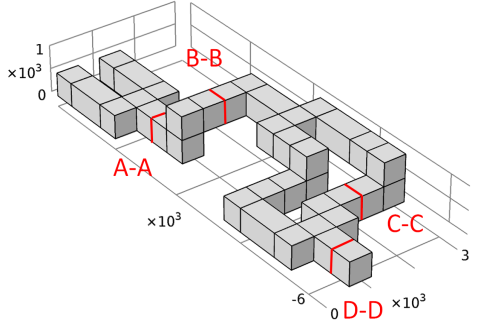
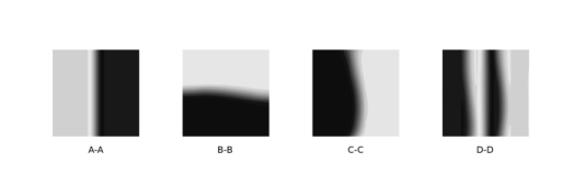
In the Model Builder window, under Results>Flow Lamination Pattern right-click Contour 2 and choose Duplicate.
2
In the Settings window for Contour, locate the Data section.
3
From the Dataset list, choose C-C.
Translation 1
1
In the Model Builder window, expand the Contour 3 node, then click Translation 1.
2
In the Settings window for Translation, locate the Translation section.
3
In the x text field, type -5*d.
4
In the y text field, type 0.
Contour 4
1
In the Model Builder window, under Results>Flow Lamination Pattern right-click Contour 3 and choose Duplicate.
2
In the Settings window for Contour, locate the Data section.
3
From the Dataset list, choose D-D.
Translation 1
1
In the Model Builder window, expand the Contour 4 node, then click Translation 1.
2
In the Settings window for Translation, locate the Translation section.
3
In the x text field, type 4.5*d.
4
In the Flow Lamination Pattern toolbar, click  Plot.
5
Click the  Zoom Extents button in the Graphics toolbar.
Flow Lamination Pattern
In the Model Builder window, under Results click Flow Lamination Pattern.
Table Annotation 1
1
In the Flow Lamination Pattern toolbar, click  More Plots and choose Table Annotation.
2
In the Settings window for Table Annotation, locate the Data section.
3
From the Source list, choose Local table.
4
5
Locate the Coloring and Style section. Clear the Show point check box.
6
From the Anchor point list, choose Center.
7
In the Flow Lamination Pattern toolbar, click  Plot.
8
Click the  Zoom Extents button in the Graphics toolbar.
9
Click the  Show Legends button in the Graphics toolbar.
10
Click the  Show Grid button in the Graphics toolbar.
Surface Average 1
Calculate the pressure drop across the mixer by adding a Surface Average feature to both inlets.
1
In the Results toolbar, click  More Derived Values and choose Average>Surface Average.
2
In the Settings window for Surface Average, locate the Selection section.
3
From the Selection list, choose Inlet.
4
Locate the Expressions section. In the table, enter the following settings:
5
Click  Evaluate.
Appendix — Geometry Instructions
From the File menu, choose New.
New
In the New window, click  Blank Model.
Add Component
In the Home toolbar, click  Add Component and choose 3D.
Geometry 1
1
In the Settings window for Geometry, locate the Units section.
2
From the Length unit list, choose mm.
Block 1 (blk1)
1
In the Geometry toolbar, click  Block.
2
In the Settings window for Block, locate the Size and Shape section.
3
In the Width text field, type 0.5.
4
In the Depth text field, type 2.
5
In the Height text field, type 0.5.
Block 2 (blk2)
1
Right-click Block 1 (blk1) and choose Duplicate.
2
In the Settings window for Block, locate the Position section.
3
In the x text field, type 1.
Block 3 (blk3)
1
Right-click Block 2 (blk2) and choose Duplicate.
2
In the Settings window for Block, locate the Position section.
3
In the x text field, type 0.5.
4
In the y text field, type -1.5.
5
Click to expand the Layers section. In the table, enter the following settings:
6
Find the Layer position subsection. Clear the Bottom check box.
7
Select the Front check box.
Block 4 (blk4)
1
Right-click Block 3 (blk3) and choose Duplicate.
2
In the Settings window for Block, locate the Size and Shape section.
3
In the Width text field, type 2.
4
In the Depth text field, type 0.5.
5
Locate the Position section. In the z text field, type 0.5.
6
Locate the Layers section. Find the Layer position subsection. Clear the Front check box.
7
Select the Left check box.
Block 5 (blk5)
1
Right-click Block 4 (blk4) and choose Duplicate.
2
In the Settings window for Block, locate the Size and Shape section.
3
In the Width text field, type 0.5.
4
In the Depth text field, type 1.5.
5
Locate the Position section. In the x text field, type 2.
6
In the y text field, type -3.
7
Locate the Layers section. Find the Layer position subsection. Clear the Left check box.
Block 6 (blk6)
1
Right-click Block 5 (blk5) and choose Duplicate.
2
In the Settings window for Block, locate the Position section.
3
In the x text field, type 1.5.
4
In the y text field, type -4.
Block 7 (blk7)
1
Right-click Block 6 (blk6) and choose Duplicate.
2
In the Settings window for Block, locate the Size and Shape section.
3
In the Depth text field, type 2.5.
4
Locate the Position section. In the y text field, type -5.
5
In the x text field, type 2.5.
Block 8 (blk8)
1
Right-click Block 7 (blk7) and choose Duplicate.
2
In the Settings window for Block, locate the Size and Shape section.
3
In the Width text field, type 2.
4
In the Depth text field, type 0.5.
5
Locate the Position section. In the x text field, type 0.
6
In the y text field, type -4.
7
In the z text field, type 0.
Block 9 (blk9)
1
Right-click Block 8 (blk8) and choose Duplicate.
2
In the Settings window for Block, locate the Position section.
3
In the x text field, type 1.
4
In the y text field, type -5.
5
Locate the Layers section. Find the Layer position subsection. Select the Left check box.
Block 10 (blk10)
1
Right-click Block 9 (blk9) and choose Duplicate.
2
In the Settings window for Block, locate the Size and Shape section.
3
In the Width text field, type 1.5.
4
Locate the Position section. In the x text field, type 0.
5
In the y text field, type -5.5.
6
Locate the Layers section. Find the Layer position subsection. Clear the Left check box.
Block 11 (blk11)
1
Right-click Block 10 (blk10) and choose Duplicate.
2
In the Settings window for Block, locate the Size and Shape section.
3
In the Width text field, type 0.5.
4
In the Depth text field, type 1.
5
Locate the Position section. In the y text field, type -5.
Block 12 (blk12)
1
Right-click Block 11 (blk11) and choose Duplicate.
2
In the Settings window for Block, locate the Position section.
3
In the x text field, type 0.5.
4
In the y text field, type -6.5.
5
Locate the Layers section. In the table, enter the following settings:
6
Find the Layer position subsection. Select the Front check box.
Partition Domains 1 (pard1)
1
In the Geometry toolbar, click  Booleans and Partitions and choose Partition Domains.
2
Click the  Select All button in the Graphics toolbar.
3
In the Settings window for Partition Domains, locate the Partition Domains section.
4
From the Partition with list, choose Extended faces.
5
Click the  Select All button in the Graphics toolbar.
Form Union (fin)
1
In the Model Builder window, click Form Union (fin).
2
In the Settings window for Form Union/Assembly, click  Build Selected.
Geometry
1
In the Geometry toolbar, click  Selections and choose Explicit Selection.
2
In the Settings window for Explicit Selection, locate the Entities to Select section.
3
From the Geometric entity level list, choose Object.
4
In the Label text field, type Geometry.
5
Inflow 1
1
In the Geometry toolbar, click  Selections and choose Explicit Selection.
2
In the Settings window for Explicit Selection, type Inflow in the Label text field.
3
Locate the Entities to Select section. From the Geometric entity level list, choose Boundary.
4
In the Label text field, type Inflow 1.
5
On the object fin, select Boundary 101 only.
Inflow 2
1
In the Geometry toolbar, click  Selections and choose Explicit Selection.
2
In the Settings window for Explicit Selection, type Inflow 2 in the Label text field.
3
Locate the Entities to Select section. From the Geometric entity level list, choose Boundary.
4
On the object fin, select Boundary 26 only.
Outlet
1
In the Geometry toolbar, click  Selections and choose Explicit Selection.
2
In the Settings window for Explicit Selection, type Outlet in the Label text field.
3
Locate the Entities to Select section. From the Geometric entity level list, choose Boundary.
4
On the object fin, select Boundary 28 only.
Inlet
1
In the Geometry toolbar, click  Selections and choose Union Selection.
2
In the Settings window for Union Selection, type Inlet in the Label text field.
3
Locate the Geometric Entity Level section. From the Level list, choose Boundary.
4
Locate the Input Entities section. Click  Add.
5
In the Add dialog box, in the Selections to add list, choose Inflow 1 and Inflow 2.
6
A-A
1
In the Geometry toolbar, click  Selections and choose Explicit Selection.
2
In the Settings window for Explicit Selection, type A-A in the Label text field.
3
Locate the Entities to Select section. From the Geometric entity level list, choose Boundary.
4
On the object fin, select Boundary 60 only.
B-B
1
In the Geometry toolbar, click  Selections and choose Explicit Selection.
2
In the Settings window for Explicit Selection, type B-B in the Label text field.
3
Locate the Entities to Select section. From the Geometric entity level list, choose Boundary.
4
On the object fin, select Boundary 125 only.
C-C
1
In the Geometry toolbar, click  Selections and choose Explicit Selection.
2
In the Settings window for Explicit Selection, type C-C in the Label text field.
3
Locate the Entities to Select section. From the Geometric entity level list, choose Boundary.
4
On the object fin, select Boundary 132 only.
D-D
1
In the Geometry toolbar, click  Selections and choose Explicit Selection.
2
In the Settings window for Explicit Selection, type D-D in the Label text field.
3
Locate the Entities to Select section. From the Geometric entity level list, choose Boundary.
4
On the object fin, select Boundary 32 only.
Walls - exterior
1
In the Geometry toolbar, click  Selections and choose Adjacent Selection.
2
In the Settings window for Adjacent Selection, type Walls - exterior in the Label text field.
3
Locate the Input Entities section. Click  Add.
4
In the Add dialog box, select Geometry in the Input selections list.
5
Walls - interior
1
In the Geometry toolbar, click  Selections and choose Adjacent Selection.
2
In the Settings window for Adjacent Selection, type Walls - interior in the Label text field.
3
Locate the Input Entities section. Click  Add.
4
In the Add dialog box, select Geometry in the Input selections list.
5
6
In the Settings window for Adjacent Selection, locate the Output Entities section.
7
Clear the Exterior boundaries check box.
8
Select the Interior boundaries check box.
Mesh Control
1
In the Geometry toolbar, click  Selections and choose Difference Selection.
2
In the Settings window for Difference Selection, type Mesh Control in the Label text field.
3
Locate the Geometric Entity Level section. From the Level list, choose Boundary.
4
Locate the Input Entities section. Click  Add.
5
In the Add dialog box, select Walls - interior in the Selections to add list.
6
7
In the Settings window for Difference Selection, locate the Input Entities section.
8
9
In the Add dialog box, in the Selections to subtract list, choose A-A, B-B, C-C, and D-D.
10
Mesh Control Faces 1 (mcf1)
1
In the Geometry toolbar, click  Virtual Operations and choose Mesh Control Faces.
2
In the Settings window for Mesh Control Faces, locate the Input section.
3
From the Faces to include list, choose Mesh Control.
Exterior Walls
1
In the Geometry toolbar, click  Selections and choose Difference Selection.
2
In the Settings window for Difference Selection, type Exterior Walls in the Label text field.
3
Locate the Geometric Entity Level section. From the Level list, choose Boundary.
4
Locate the Input Entities section. Click  Add.
5
In the Add dialog box, select Walls - exterior in the Selections to add list.
6
7
In the Settings window for Difference Selection, locate the Input Entities section.
8
9
In the Add dialog box, in the Selections to subtract list, choose Outlet and Inlet.
10