
|
|
|
|
Cp
|
|||


|
1
|
|
2
|
In the Select Physics tree, select Heat Transfer>Heat Transfer in Solids (ht) and Heat Transfer>Metal Processing>Alpha-Beta Phase Transformation (abp).
|
|
3
|
Click Add.
|
|
4
|
Click
|
|
5
|
|
6
|
Click
|
|
1
|
|
2
|
|
1
|
|
2
|
|
3
|
|
1
|
|
2
|
|
3
|
|
4
|
|
5
|
|
1
|
|
2
|
|
3
|
|
4
|
|
5
|
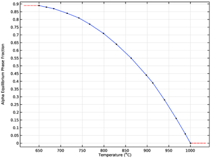
Browse to the model’s Application Libraries folder and double-click the file welding_of_a_titanium_plate_xieqalpha.txt.
|
|
6
|
|
7
|
In the Argument table, enter the following settings:
|
|
1
|
|
2
|
|
3
|
|
4
|
|
5
|
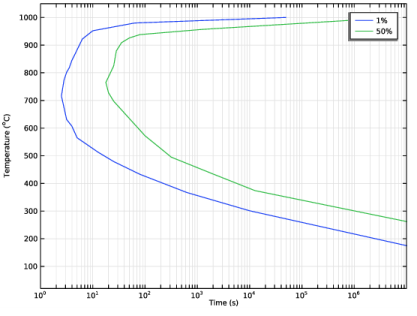
Browse to the model’s Application Libraries folder and double-click the file welding_of_a_titanium_plate_ttt1.txt.
|
|
6
|
|
7
|
|
8
|
In the Argument table, enter the following settings:
|
|
1
|
|
2
|
|
3
|
|
4
|
|
5
|
Browse to the model’s Application Libraries folder and double-click the file welding_of_a_titanium_plate_ttt50.txt.
|
|
6
|
|
7
|
|
8
|
In the Argument table, enter the following settings:
|
|
1
|
|
2
|
|
3
|
|
4
|
|
5
|
Browse to the model’s Application Libraries folder and double-click the file welding_of_a_titanium_plate_fdiss.txt.
|
|
6
|
|
7
|
In the Argument table, enter the following settings:
|
|
1
|
|
2
|
|
3
|
|
4
|
|
5
|
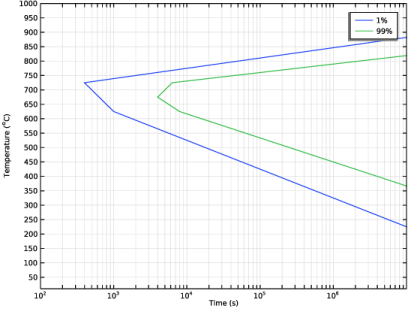
Browse to the model’s Application Libraries folder and double-click the file welding_of_a_titanium_plate_ttt1m.txt.
|
|
6
|
|
7
|
|
8
|
In the Argument table, enter the following settings:
|
|
1
|
|
2
|
|
3
|
|
4
|
|
5
|
Browse to the model’s Application Libraries folder and double-click the file welding_of_a_titanium_plate_ttt99m.txt.
|
|
6
|
|
7
|
|
8
|
In the Argument table, enter the following settings:
|
|
1
|
|
2
|
|
3
|
|
4
|
|
1
|
|
2
|
|
3
|
|
4
|
|
1
|
|
2
|
|
3
|
|
4
|
|
1
|
|
2
|
|
3
|
|
4
|
|
1
|
|
2
|
|
3
|
|
4
|
|
5
|
|
6
|
|
7
|
|
8
|
|
9
|
Clear the Bottom check box.
|
|
11
|
|
1
|
In the Model Builder window, under Component 1 (comp1) right-click Heat Transfer in Solids (ht) and choose Heat Source.
|
|
2
|
|
3
|
|
4
|
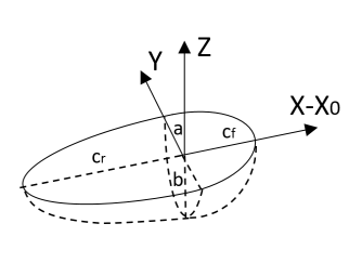
Locate the Heat Source section. In the Q0 text field, type (X>=X0)*an1(X-X0,Y,Z,q0,a,b,cf) + (X<X0)*an1(X-X0,Y,Z,q0,a,b,cr).
|
|
1
|
|
3
|
|
4
|
|
5
|
|
6
|
|
1
|
|
3
|
In the Settings window for Surface-to-Ambient Radiation, locate the Surface-to-Ambient Radiation section.
|
|
4
|
|
1
|
|
2
|
|
3
|
|
1
|
In the Model Builder window, under Component 1 (comp1)>Alpha-Beta Phase Transformation (abp) click Beta.
|
|
2
|
|
3
|
|
1
|
|
2
|
|
3
|
|
1
|
|
2
|
|
3
|
|
1
|
|
2
|
|
3
|
|
4
|
|
5
|
|
6
|
|
7
|
|
8
|
|
1
|
|
2
|
|
3
|
|
1
|
|
2
|
|
3
|
|
4
|
|
5
|
|
6
|
|
7
|
|
1
|
|
2
|
|
3
|
|
4
|
|
5
|
|
6
|
|
7
|
|
1
|
|
2
|
|
3
|
|
4
|
|
5
|
|
1
|
|
2
|
Right-click Global Definitions>Materials>Beta (abpphase1mat)>Basic (def) and choose Functions>Analytic.
|
|
3
|
|
4
|
|
5
|
|
6
|
|
8
|
|
1
|
In the Model Builder window, under Global Definitions>Materials>Beta (abpphase1mat) click Basic (def).
|
|
2
|
|
4
|
|
5
|
|
6
|
Click OK.
|
|
7
|
|
1
|
|
2
|
|
3
|
|
4
|
|
5
|
|
6
|
Locate the Units section. In the table, enter the following settings:
|
|
7
|
|
1
|
In the Model Builder window, under Global Definitions>Materials>Beta (abpphase1mat) click Basic (def).
|
|
2
|
|
1
|
|
2
|
Right-click Global Definitions>Materials>Widmanstätten Alpha (abpphase2mat)>Basic (def) and choose Functions>Analytic.
|
|
3
|
|
4
|
|
5
|
|
6
|
|
8
|
|
1
|
In the Model Builder window, under Global Definitions>Materials>Widmanstätten Alpha (abpphase2mat) click Basic (def).
|
|
2
|
|
4
|
|
5
|
|
6
|
Click OK.
|
|
7
|
|
1
|
|
2
|
|
3
|
|
4
|
|
5
|
Locate the Units section. In the table, enter the following settings:
|
|
6
|
|
1
|
In the Model Builder window, under Global Definitions>Materials>Widmanstätten Alpha (abpphase2mat) click Basic (def).
|
|
2
|
|
1
|
|
2
|
Right-click Global Definitions>Materials>Martensitic Alpha (abpphase3mat)>Basic (def) and choose Functions>Analytic.
|
|
3
|
|
4
|
|
5
|
|
6
|
|
8
|
|
1
|
In the Model Builder window, under Global Definitions>Materials>Martensitic Alpha (abpphase3mat) click Basic (def).
|
|
2
|
|
4
|
|
5
|
|
6
|
Click OK.
|
|
7
|
|
1
|
|
2
|
|
3
|
|
4
|
|
5
|
Locate the Units section. In the table, enter the following settings:
|
|
6
|
|
1
|
In the Model Builder window, under Global Definitions>Materials>Martensitic Alpha (abpphase3mat) click Basic (def).
|
|
2
|
|
1
|
|
1
|
|
2
|
|
3
|
|
1
|
|
1
|
|
2
|
|
3
|
|
1
|
|
2
|
|
3
|
|
4
|
|
1
|
|
2
|
|
3
|
|
4
|
|
1
|
|
2
|
|
3
|
|
4
|
|
5
|
|
6
|
|
7
|
Click
|
|
1
|
|
2
|
|
3
|
|
4
|
|
5
|
|
6
|
|
1
|
|
2
|
In the Settings window for Point Graph, click Replace Expression in the upper-right corner of the y-Axis Data section. From the menu, choose Component 1 (comp1)>Alpha-Beta Phase Transformation>Phase composition>abp.phase1.xi - Phase fraction.
|
|
3
|
|
4
|
|
1
|
|
2
|
In the Settings window for Point Graph, click Replace Expression in the upper-right corner of the y-Axis Data section. From the menu, choose Component 1 (comp1)>Alpha-Beta Phase Transformation>Phase composition>abp.phase2.xi - Phase fraction.
|
|
3
|
|
4
|
|
1
|
|
2
|
In the Settings window for Point Graph, click Replace Expression in the upper-right corner of the y-Axis Data section. From the menu, choose Component 1 (comp1)>Alpha-Beta Phase Transformation>Phase composition>abp.phase3.xi - Phase fraction.
|
|
3
|
|
4
|
|
1
|
|
2
|
|
3
|
|
4
|
|
5
|
|
6
|
|
8
|
Click to expand the Coloring and Style section. Find the Line style subsection. From the Line list, choose Dashed.
|
|
9
|