Thermoelastic Damping in a MEMS Resonator

High quality factor MEMS resonators are the key components in the emerging MEMS timing industry. In these applications a MEMS resonator is driven at its resonant frequency by a feedback loop to produce a circuit that oscillates at a fixed frequency. Such frequency references are used in a huge range of electronic devices, from CPU clocks to mobile phones. For oscillator applications the quality factor of the resonator, together with the stability of the resonant frequency, determines the ultimate performance achievable. Higher quality factor resonators have a sharper peak in their frequency spectrum at the resonant frequency and therefore pick out a particular frequency with higher fidelity. For many resonant modes the limit to the achievable quality factor is determined by thermoelastic damping.

To understand thermoelastic damping consider the stretching of a thermally isolated elastic rod. When such a rod is stretched uniformly and reversibly its temperature drops. The drop in temperature compensates for the increase in entropy caused by the stress in the rod (since the process is reversible the entropy remains constant). Similarly on compression the rod heats up. When a structure vibrates in a more complex normal mode there are some regions of compression and some of extension. Depending on the time scale of the vibration, heat flows from the warmer parts of the structure to the cooler parts. Since heat flow is an irreversible process, this heat flow is associated with energy loss from the vibrational mode, and corresponding damping for the resonant mode. Thermoelastic damping is particularly important in smaller MEMS structures, in which regions of compression and expansion are in close proximity.

Model Definition

The model consists of a single beam vibrating in its fundamental mode, perpendicular to its long axis. The model geometry is shown in Figure 1. The two ends of the beam are fixed and are assumed to be connected to a much larger body (for example, a contact pad), which acts as a thermal reservoir.

Figure 1: Symmetric model geometry. The geometry consists of a silicon beam 12 μm thick and 400 μm long. The beam width is 20 μm but since the geometry is symmetric only half of the beam width is shown and the symmetry boundary conditions is used. The two ends of the beam are assumed to be clamped to a body with a large thermal mass, such as a contact pad.

This analysis computes the resonator quality factor, assuming that thermoelastic damping is the dominant damping mechanism. The coupled equations of thermoelasticity are solved within the resonator.

Derivation of the thermoelasticity equations

References 1 to 7 provide useful background information.

The equations of thermoelasticity are derived from the first law of thermodynamics, which can be stated as follows:

(1)

where dU is the change in internal energy, dQ' is the heat flow into the system (the prime indicates an inexact differential in this case) and dW' is the work done on the system. For a small part of a solid (sufficiently small that the stresses and strains are uniform), with an initial reference density, ρ0, the first law can be rewritten in the following form (assuming that the differential changes occur between equilibrium states):

(2)

where Ta is the absolute temperature, s is the entropy per unit mass, σ is the elastic part of the second Piola-Kirchhoff stress (in general a rank 2 tensor), ε is the material strain (also a tensor). In general the second Piola-Kirchhoff stress tensor, p, must be split into elastic (σ) and inelastic (τ) parts such that:

The elastic part of the stress tensor, σ, does work σ:dε during a change in the strain. The inelastic part of the strain tensor, τ, generates heat at a rate τ:(dε/dτ) when the strain is changing and is identified with internal or material damping. These internal damping mechanisms are associated with microscopic phenomena such as dislocation movement.

From Equation 2 it is possible to make the following identifications for Ta and σ:

Next the entropy balance equation must be derived. Because thermoelasticity involves irreversible processes, the assumption of equilibrium required to derive Equation 2 is no longer valid. Instead an assumption of ‘local’ equilibrium is made. It is assumed that although the system is not in equilibrium, there exists within small elements a state of local equilibrium, for which the local entropy per unit mass, s, is the same function of the internal energy, strain, and particle number as it was in equilibrium. This assumption is commonly employed in the modeling of transport phenomena and is justified only by the validity of conclusions derived from it and by results obtained from specific microscopic models, for near-equilibrium situations. For a small volume element in the material frame Equation 2 can then be written as

The rate of change of entropy can then be written as

(3)

From the first law (Equation 1) the rate of change of internal energy is given by:

where w is the work done per unit volume and q is the heat accumulated per unit volume. The heat accumulated can be written as the sum of the heat sources and the divergence in the material frame heat flux:

where Q represents the heat source per unit volume and τ is the inelastic part of the stress tensor. The rate of doing work (per unit reference volume) by a linear elastic material is given by the elastic part of the second Piola-Kirchhoff stress contracted with the rate of material strain. Per unit volume the following equation is obtained:

so Equation 3 reduces to

The definition of the material thermal conductivity gives

where κ is the thermal conductivity, defined in the material frame.

Therefore the equation is

(4)

It is now necessary to derive an expression for the rate of change of entropy with respect to time. In order to do this an assumption of local equilibrium is used once again. Using Equation 2 the equation is written

which defines a new thermodynamic potential, the Gibbs free energy per unit mass, given by

Changes in the Gibbs free energy per unit mass take the form

which leads to the relations

By differentiating each of the above equations a second time, it is possible to derive the following Maxwell relation

(5)

It is now possible to derive an expression for the entropy of the solid. Assuming that the elastic stress is an invertible function of the strain, we can write s=s(σ,Ta). Thus,

Using the Maxwell relation in Equation 5 gives

so that

By definition the heat capacity of the solid at constant stress is given by

Thus,

(6)

Substituting Equation 6 into Equation 4 gives the following equation for thermoelasticity:

(7)

An additional heat source term is present in Equation 7, compared to the standard heat transfer equations in solids. This term couples the structural problem with the heat transfer problem. In turn the heat transfer equation couples back into the structural problem through the constitutive relationship. The COMSOL Multiphysics software solves a linearized form of the anisotropic thermoelasticity equations given in Equation 7.

In the particular case of a linear elastic material (in the absence of damping) the stress and strain are related by Duhamel-Hooke’s law:

where C is the elasticity tensor, σi is the initial stress, εi is the initial strain and Tref is the reference temperature at which the strain and stresses take the initial values.

This equation couples the heat transfer equation to the structural problem. Given a temperature independent thermal expansivity, and no material damping, Equation 7 takes the form

which is the usual form of the equation for linear thermoelasticity.

Results and Discussion

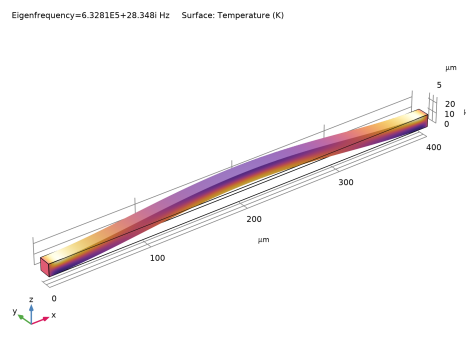
Figure 2 shows the mode shape and the corresponding temperature distribution within the beam. The mode has an eigenfrequency of 63.3 kHz and a quality factor of 10700. In Ref. 4 Zener derived an approximate analytic expression for the quality factor of a thin isotropic beam vibrating in its fundamental mode, by considering only the thermal gradients in the direction of flexure. Zener’s expression is given by:

(8)

where E is the Young’s modulus of the beam, α is the isotropic thermal expansivity, ω is the mechanical angular resonant frequency and τ is the thermal relaxation time constant of the system, given by:

where h is the beam thickness and κ is the thermal conductivity of the mode. The resonant frequency of the beam can also be computed analytically and is given by:

(9)

Table 1 compares the COMSOL Multiphysics model with values computed using Equation 8 and Equation 9 and with experimental results, obtained from Ref. 7. Note that the COMSOL Multiphysics model has a slightly higher quality factor than the theoretical result because some of the thermal gradients are removed by the isothermal boundary condition (the quality factor is reduced significantly if a thermal insulation boundary condition is applied to the end boundaries — in practice the real boundary condition is somewhere between these two extremes).

Figure 2: Fundamental mode shape and corresponding temperature distribution within the beam.

Table 1: Comparison of results from the model with theory and experiment.
Source	Resonant Frequency (MHz)	Quality factor
COMSOL Model	0.63	11.2×103
Equation 8 and Equation 9	0.63	10.3×103
Experiment (Ref. 7)	0.57	10.3×103

References

1. C.J. Adkins, Equilibrium Thermodynamics, Cambridge University Press, 1983.

2. W. Yourgrau, A. van der Merwe, and G. Raw, Treatise on Irreversible and Statistical Thermodynamics: An Introduction to Nonclassical Thermodynamics, Dover Publications, Inc., New York, 2002.

3. C. Zener, “Internal Friction in Solids I: Theory of Internal Friction in Reeds,” Physical Review, vol. 52, pp. 90–99, 1937.

4. C. Zener, “Internal Friction in Solids II: General Theory of Thermoelastic Internal Friction,” Physical Review, vol. 53, pp. 230–235, 1938.

5. M. E. Gurtin, E. Fied, and L. Anand, The Mechanics and Thermodynamics of Continua, Cambridge University Press, 2010.

6. V.A. Lubarda, “On Thermodynamic Potentials in Linear Thermoelasticity,” Int. J. Solids and Structures, vol. 41, no. 26, pp. 7377–7398, 2004.

7. A. Duwel, R.N. Candler, T.W. Kenny, and M. Varghese, “Engineering MEMS Resonators with Low Thermoelastic Damping,” J. Microelectromechanical Systems, vol. 15, no. 6, pp. 1437–1445, 2006.

MEMS_Module/Actuators/thermoelastic_damping_3d

Modeling Instructions

From the menu, choose .

New

In the window, click

Model Wizard

In the window, click

In the tree, select .

Click .

Click

In the tree, select .

Click

Geometry 1

The Model Wizard led to the node in the Model Builder tree structure. Start building the simple beam structure by specifying a convenient length unit.

In the window, under click .

In the window for , locate the section.

From the list, choose .

Block 1 (blk1)

In the toolbar, click

In the window for , locate the section.

In the text field, type 400.

In the text field, type 12.

Click

Import material parameters from a file.

Global Definitions

Parameters 1

In the window, under click .

In the window for , locate the section.

Click

Browse to the model’s Application Libraries folder and double-click the file thermoelastic_damping_3d_parameters.txt.

Create a blank material and fill in the material properties using the parameters that we just imported.

Materials

Material 1 (mat1)

In the window, under right-click and choose .

In the window for , locate the section.

In the table, enter the following settings:


Property	Variable	Value	Unit	Property group
Young’s modulus	E	E0	Pa	Young’s modulus and Poisson’s ratio
Poisson’s ratio	nu	nu0	1	Young’s modulus and Poisson’s ratio
Density	rho	rho0	kg/m³	Basic
Thermal conductivity	k_iso ; kii = k_iso, kij = 0	kappa0	W/(m·K)	Basic
Heat capacity at constant pressure	Cp	Cp0	J/(kg·K)	Basic
Coefficient of thermal expansion	alpha_iso ; alphaii = alpha_iso, alphaij = 0	alpha0	1/K	Basic