PDF

Pyroelectric Detector
Introduction
The pyroelectric phenomenon, when absorbed energy causes a change in temperature and polarization within a pyroelectric material, is the basis of operation of some laser energy meters. The change in polarization manifests itself as a pyroelectric current, which can be measured by an ammeter circuit. Laser energy meters based on the pyroelectric phenomenon are used to calibrate of laser sources.
This 2D axisymmetric model demonstrates the operation of a pyroelectric detector based on a lithium niobate (LiNbO3) crystal sandwiched between two electrodes with connection to an external circuit. To represent the absorbed laser energy, an energy flux that varies with position and time is applied to the top surface of the disk. This model uses (i) the Piezoelectricity and Pyroelectricity multiphysics interface and (ii) the Electrical Circuit interface. A time-dependent study solves for temperature evolution in the disk and the pyroelectric current generated.
Model Definition
A 25 μm-thick LiNbO3 crystal in the shape of a disk with a diameter of 3 mm is bonded to an electrically conductive base by a 40 μm thick ring-shaped silver (Ag) pad. Most material properties of the LiNbO3 and Ag domains are defined by material models from the material library and some properties need to be added manually. The pyroelectric coefficient of LiNbO3 was specified as 83 μC/(m2·K). The top and bottom surfaces of the crystal are coated with a thin metal layer, forming the top and bottom electrodes. The model geometry is fully parameterized to allow for easy changes in the device structure for future optimization.
This model uses the Piezoelectricity and Pyroelectricity multiphysics interface, which automatically sets up the Electrostatics, Solid Mechanics, and Heat Transfer interfaces together with Pyroelectricity, Piezoelectric Effect, and Thermal Expansion couplings. In the Electrostatics interface, a Charge Conservation, Piezoelectric material model is assigned to the LiNbO3 domain. In the Solid Mechanics interface, a Fixed Constraint is applied to the base of the Ag pad. In the Heat Transfer interface, an Heat Flux applied to the top surface of the disk represents the laser energy while a constant temperature of 293.15 K is assigned to the base of the Ag pad. These assignments can be seen in Figure 1.
Figure 1: A cross section of the 2D axi-symmetric model showing the material models and boundary conditions used. The disk is lithium niobate (purple) and the pad is silver (gray). The bottom surface of the disk is grounded (yellow) while the top electrode (red) is connected to an external circuit. A fixed constraint and T = 293.15 K is applied to the bottom of the silver pad.
To calculate output power, the device is connected to an external circuit using the Electrical Circuit interface. The terminals of the LiNbO3 disk is connected in parallel to the capacitor C1 with a capacitance value of Cext = 100 pF. The disk is also connected to the load R1 with resistance value of Rext = 0.1, 5.106, 5.107, or 109 Ω. The electrical power is calculated as the product of the voltage and current across R1. The circuit components are parameterized to allow for easy changes in the device structure for future optimization.
The model solves a multiphysics problem involving Pyroelectricity, Piezoelectric Effect, and Thermal Expansion couplings using a time-dependent study. In the first study, the model includes all couplings and is referred to as the full model. In the second study, the Piezoelectric Effect and Thermal Expansion couplings are disabled, and the model is referred to as pyroelectricity-only.
Results and Discussion
A plot of temperature and current through R1versus time is shown in Figure 2 with the temperature measured at the center of the disk.
Figure 2: Temperature and current through R1 versus time at the center of the disk.
Figure 3 shows a plot of voltage versus time with the voltage measurements taken across the load R1.
Figure 3: Voltage versus time. Voltage measurements taken across the load R1.
Figure 4 shows a plot of electric power versus time, with the electric power measurements taken through the load R1.
Figure 4: Electric power versus time. Electric power measurements taken through the load R1.
Figure 5 shows a comparison of the electric power between the full model and the pyroelectricity-only model. The electric power for the full model is about 8% less than for the pyroelectricity-only model.
Figure 5: Comparison of electric power between full model and pyroelectricity-only model.
Application Library path: MEMS_Module/Sensors/pyroelectric_detector
Modeling Instructions
Start by creating a new 2D axi-symmetric model with the Piezoelectricity and Pyroelectricity multiphysics interface and the Electrical Circuit interface.
From the File menu, choose New.
New
In the New window, click  Model Wizard.
Model Wizard
1
In the Model Wizard window, click  2D Axisymmetric.
2
In the Select Physics tree, select AC/DC>Electromagnetics and Mechanics>Piezoelectricity>Piezoelectricity and Pyroelectricity.
3
Click Add.
4
In the Select Physics tree, select AC/DC>Electrical Circuit (cir).
5
Click Add.
6
Click  Study.
7
In the Select Study tree, select General Studies>Time Dependent.
8
Define and enter the values for the following global parameters.
Global Definitions
Parameters 1
1
In the Model Builder window, under Global Definitions click Parameters 1.
2
In the Settings window for Parameters, locate the Parameters section.
3
Define a rectangular function and an analytical function describing the shape of laser pulse.
Definitions
Rectangle 1 (rect1)
1
In the Home toolbar, click  Functions and choose Local>Rectangle.
2
In the Settings window for Rectangle, locate the Parameters section.
3
In the Lower limit text field, type 0.2.
4
In the Upper limit text field, type 1.
Analytic 1 (an1)
1
In the Home toolbar, click  Functions and choose Local>Analytic.
2
In the Settings window for Analytic, locate the Definition section.
3
In the Expression text field, type exp(-((r^2)/(2*(10000)^2))).
4
In the Arguments text field, type r.
5
Locate the Units section. In the table, enter the following settings:
Define the expression for the energy flux representing laser pulse using the functions previously defined.
Variables 1
1
In the Model Builder window, right-click Definitions and choose Variables.
2
In the Settings window for Variables, locate the Variables section.
3
Geometry 1
1
In the Model Builder window, under Component 1 (comp1) click Geometry 1.
2
In the Settings window for Geometry, locate the Units section.
3
From the Length unit list, choose mm.
Rectangle 1 (r1)
1
In the Geometry toolbar, click  Rectangle.
2
In the Settings window for Rectangle, locate the Size and Shape section.
3
In the Width text field, type r_d.
4
In the Height text field, type t_d.
Rectangle 2 (r2)
1
In the Geometry toolbar, click  Rectangle.
2
In the Settings window for Rectangle, locate the Size and Shape section.
3
In the Width text field, type r_s.
4
In the Height text field, type t_s.
5
Locate the Position section. In the r text field, type r_d-0.3.
6
In the z text field, type -t_p.
7
In the r text field, type r_d-r_s.
8
In the z text field, type -t_s.
Rectangle 3 (r3)
1
In the Geometry toolbar, click  Rectangle.
2
In the Settings window for Rectangle, locate the Size and Shape section.
3
In the Width text field, type r_el.
4
In the Height text field, type t_d.
5
Click  Build Selected.
Multiphysics
Pyroelectricity 1 (pye1)
1
In the Model Builder window, under Component 1 (comp1)>Multiphysics click Pyroelectricity 1 (pye1).
2
Add the lithium niobate model from the library.
Add Material
1
In the Home toolbar, click  Add Material to open the Add Material window.
2
Go to the Add Material window.
3
In the tree, select Piezoelectric>Lithium Niobate.
4
Click Add to Component in the window toolbar.
5
In the Home toolbar, click  Add Material to close the Add Material window.
Materials
Lithium Niobate (mat1)
Next, enter missing properties for lithium niobate.
1
In the Settings window for Material, locate the Material Contents section.
2
Setup the boundary conditions for the Electrostatics interface.
Electrostatics (es)
Charge Conservation, Piezoelectric 1
1
In the Model Builder window, under Component 1 (comp1)>Electrostatics (es) click Charge Conservation, Piezoelectric 1.
2
Ground 1
1
In the Physics toolbar, click  Boundaries and choose Ground.
2
Terminal 1
1
In the Physics toolbar, click  Boundaries and choose Terminal.
2
In the Settings window for Terminal, locate the Boundary Selection section.
3
Click  Paste Selection.
4
In the Paste Selection dialog box, type 3 in the Selection text field.
5
6
In the Settings window for Terminal, locate the Terminal section.
7
From the Terminal type list, choose Circuit.
Charge Conservation 1
1
In the Model Builder window, click Charge Conservation 1.
2
In the Settings window for Charge Conservation, locate the Material Type section.
3
From the Material type list, choose Solid.
Solid Mechanics (solid)
Piezoelectric Material 1
1
In the Model Builder window, under Component 1 (comp1)>Solid Mechanics (solid) click Piezoelectric Material 1.
2
Setup the boundary conditions for the Solid Mechanics interface.
Fixed Constraint 1
1
In the Physics toolbar, click  Boundaries and choose Fixed Constraint.
2
Setup the boundary conditions for the Heat Transfer interface.
Heat Transfer in Solids (ht)
In the Model Builder window, under Component 1 (comp1) click Heat Transfer in Solids (ht).
Heat Flux 1
1
In the Physics toolbar, click  Boundaries and choose Heat Flux.
2
In the Settings window for Heat Flux, locate the Material Type section.
3
From the Material type list, choose Solid.
4
Locate the Heat Flux section. In the q0 text field, type Flux.
5
Temperature 1
1
In the Physics toolbar, click  Boundaries and choose Temperature.
2
Add the Electric Circuit interface, define the capacitor C_ext and the load R_ext and how they are connected to the detector terminals.
Electrical Circuit (cir)
In the Model Builder window, under Component 1 (comp1) click Electrical Circuit (cir).
Resistor 1 (R1)
1
In the Electrical Circuit toolbar, click  Resistor.
2
In the Settings window for Resistor, locate the Node Connections section.
3
4
Locate the Device Parameters section. In the R text field, type R_ext.
Capacitor 1 (C1)
1
In the Electrical Circuit toolbar, click  Capacitor.
2
In the Settings window for Capacitor, locate the Node Connections section.
3
4
Locate the Device Parameters section. In the C text field, type C_ext.
External I-terminal 1 (termI1)
1
In the Electrical Circuit toolbar, click  External I-terminal.
2
In the Settings window for External I-terminal, locate the Node Connections section.
3
In the Node name text field, type 1.
4
Locate the External Terminal section. From the V list, choose Terminal voltage (es/term1).
Add material model for silver.
Add Material
1
In the Home toolbar, click  Add Material to open the Add Material window.
2
Go to the Add Material window.
3
In the tree, select MEMS>Metals>Ag - Silver.
4
Click Add to Component in the window toolbar.
5
In the Home toolbar, click  Add Material to close the Add Material window.
Materials
Ag - Silver (mat2)
Next, enter missing properties for silver.
1
2
In the Settings window for Material, locate the Material Contents section.
3
4
Click the  Zoom Extents button in the Graphics toolbar.
Mesh 1
Free Triangular 1
In the Mesh toolbar, click  Free Triangular.
Size 1
1
Right-click Free Triangular 1 and choose Size.
2
In the Settings window for Size, locate the Element Size section.
3
From the Predefined list, choose Extremely fine.
4
Click  Build Selected.
Add a time-dependent study using the full model to analyze effect of thermal expansion, piezoelectricity and pyroelectricity.
Study 1
Time Dependent, Full Model
1
In the Model Builder window, under Study 1 click Step 1: Time Dependent.
2
In the Settings window for Time Dependent, locate the Study Settings section.
3
In the Output times text field, type range(0,0.02,2).
4
In the Label text field, type Time Dependent, Full Model.
5
Click to expand the Study Extensions section. Select the Auxiliary sweep check box.
6
7
8
In the Model Builder window, click Study 1.
9
In the Settings window for Study, locate the Study Settings section.
10
Clear the Generate default plots check box.
11
In the Home toolbar, click  Compute.
Add a time-dependent study using the pyroelectricity-only model to analyze effect of pyroelectricity.
Add Study
1
In the Home toolbar, click  Add Study to open the Add Study window.
2
Go to the Add Study window.
3
Find the Studies subsection. In the Select Study tree, select General Studies>Time Dependent.
4
Click Add Study in the window toolbar.
Study 2
Time Dependent - Pyroelectricity Only
1
In the Settings window for Time Dependent, type Time Dependent - Pyroelectricity Only in the Label text field.
2
Locate the Study Settings section. In the Output times text field, type range(0,0.02,2).
3
Locate the Physics and Variables Selection section. In the table, enter the following settings:
4
5
Locate the Study Extensions section. Select the Auxiliary sweep check box.
6
7
8
In the Model Builder window, click Study 2.
9
In the Settings window for Study, locate the Study Settings section.
10
Clear the Generate default plots check box.
11
In the Home toolbar, click  Compute.
Plot temperature and current density versus time, taking measurement at the center of the disk.
Results
Temperature and Current Density, Full Model
1
In the Home toolbar, click  Add Plot Group and choose 1D Plot Group.
2
In the Settings window for 1D Plot Group, type Temperature and Current Density, Full Model in the Label text field.
3
Locate the Plot Settings section. Select the Two y-axes check box.
Temperature
1
Right-click Temperature and Current Density, Full Model and choose Point Graph.
2
Click the  Zoom Extents button in the Graphics toolbar.
3
4
In the Settings window for Point Graph, locate the y-Axis Data section.
5
In the Expression text field, type T.
6
Select the Description check box.
7
In the Temperature and Current Density, Full Model toolbar, click  Plot.
8
In the Label text field, type Temperature.
Circuit Current
1
In the Model Builder window, right-click Temperature and Current Density, Full Model and choose Global.
2
In the Settings window for Global, type Circuit Current in the Label text field.
3
Locate the y-Axis section. Select the Plot on secondary y-axis check box.
4
Locate the y-Axis Data section. In the table, enter the following settings:
5
Click to expand the Legends section. Find the Include subsection. Clear the Description check box.
6
In the Temperature and Current Density, Full Model toolbar, click  Plot.
Temperature and Current Density, Full Model
1
In the Model Builder window, click Temperature and Current Density, Full Model.
2
In the Settings window for 1D Plot Group, locate the Plot Settings section.
3
In the table, select the Plot on secondary y-axis check box for Circuit Current.
4
In the Temperature and Current Density, Full Model toolbar, click  Plot.
Plot voltage versus time, taking measurement across the load R_ext.
Voltage, Full Model
1
In the Home toolbar, click  Add Plot Group and choose 1D Plot Group.
2
In the Settings window for 1D Plot Group, type Voltage, Full Model in the Label text field.
3
Locate the Legend section. From the Position list, choose Lower right.
Global 1
1
Right-click Voltage, Full Model and choose Global.
2
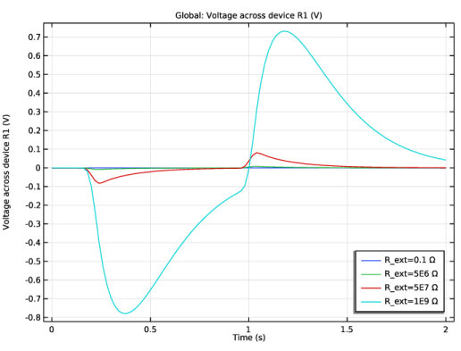
In the Settings window for Global, click Replace Expression in the upper-right corner of the y-Axis Data section. From the menu, choose Component 1 (comp1)>Electrical Circuit>Devices>R1>cir.R1_v - Voltage across device R1 - V.
3
Locate the Legends section. Find the Include subsection. Clear the Description check box.
4
In the Voltage, Full Model toolbar, click  Plot.
Plot electric power versus time, taking measurement across the load R_ext.
Electric Power, Full Model
1
In the Home toolbar, click  Add Plot Group and choose 1D Plot Group.
2
In the Settings window for 1D Plot Group, type Electric Power, Full Model in the Label text field.
Global 1
1
Right-click Electric Power, Full Model and choose Global.
2
In the Settings window for Global, locate the y-Axis Data section.
3
4
Locate the Legends section. Find the Include subsection. Clear the Description check box.
5
In the Electric Power, Full Model toolbar, click  Plot.
Plot electric power versus time for R_ext = 1e9 ohms for the full model and the pyroelectricity-only model.
Full Model vs. Pyroelectricity Only
1
In the Home toolbar, click  Add Plot Group and choose 1D Plot Group.
2
In the Settings window for 1D Plot Group, type Full Model vs. Pyroelectricity Only in the Label text field.
Electric Power, Full Model
1
Right-click Full Model vs. Pyroelectricity Only and choose Global.
2
In the Settings window for Global, type Electric Power, Full Model in the Label text field.
3
Locate the Data section. From the Dataset list, choose Study 1/Solution 1 (sol1).
4
From the Parameter selection (R_ext) list, choose From list.
5
In the Parameter values (R_ext (Ω)) list, select 1E9.
6
Locate the y-Axis Data section. In the table, enter the following settings:
7
Locate the Legends section. Find the Include subsection. Clear the Solution check box.
Electric Power, Pyroelectricity Only
1
Right-click Electric Power, Full Model and choose Duplicate.
2
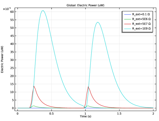
In the Settings window for Global, type Electric Power, Pyroelectricity Only in the Label text field.
3
Locate the Data section. From the Dataset list, choose Study 2/Solution 2 (sol2).
4
Locate the y-Axis Data section. In the table, enter the following settings:
5
In the Full Model vs. Pyroelectricity Only toolbar, click  Plot.