PDF

Piezoelectric Energy Harvester
Introduction
The development of extremely low power electronics and wireless systems has led to a strong interest in the field of energy harvesting — the development of miniature generators. Typically these devices are used to power sensors and wireless communication systems, enabling standalone ‘wireless sensors’ that are cheap to deploy. Frequently wireless sensors make measurements intermittently over an extended period, reporting via a wireless link to other sensors and ultimately to a base station that records readings from all the deployed sensors (creating a ‘wireless sensor network’). This model analyzes a simple "seismic" energy harvester, that is designed to generate electrical energy from local variations in acceleration, that occur, for example, when a wireless sensor is mounted on a vibrating piece of machinery. The energy harvester analyzed in this model consists of a piezoelectric bimorph clamped at one end to the vibrating machinery with a proof mass mounted on its other end. It is loosely based on the mechanical system described in detail in Ref. 1.
Model Definition
Figure 1 shows the device geometry. The power harvester consists of a piezoelectric bimorph clamped at one end with a proof mass mounted on the other end. The bimorph has two output electrodes embedded within it and two ground electrodes on the exterior surfaces of the cantilever beam. This configuration ensures that same voltage is induced on the output electrodes, even though the stress above and below the neutral layer is of opposite sign. Since the clamp is mounted to a piece of vibrating machinery the device is analyzed in a vibrating reference frame (modeled in COMSOL by the application of a sinusoidal body load).
Figure 1: 2D model geometry, showing the major components of the energy harvester, including the piezoelectric bimorph, proof mass and supporting structure.
The model performs three analyses of the mechanical part of the energy harvester system. First, the power output is analyzed as a function of vibration frequency, with a fixed electrical load. Then the power output as a function of electrical load is explored. Finally the DC voltage output, as a function of acceleration, is shown to be linear.
Results and Discussion
Figure 2 shows the input mechanical power and the power harvested (in mW) as well as the peak voltage induced across the piezoelectric bimorph (in V) as a function of frequency when the energy harvester is excited by a sinusoidal acceleration. The electrical load is 12 kΩ. The response of the system shows a peak at 76Hz, close to the computed resonant frequency of the cantilever at 73 Hz (from a separate eigenfrequency analysis of this device).
Figure 2: Energy harvester input mechanical power and the power harvested (in mW) as well as the peak voltage induced across the piezoelectric bimorph (in V) vs. excitation frequency. The load impedance is 12 kΩ and the acceleration magnitude is 1 g.
Figure 3: Power harvested from the device as a function of the electrical load resistance at an acceleration of 1 g oscillating at 75.5Hz.
Figure 3 shows the harvested power from the device as a function of the electrical load resistance at an acceleration of 1 g oscillating at 75.5Hz. The peak in energy harvested corresponds to an electrical load of 6 kΩ.
Figure 4: DC voltage and mechanical/electrical power output versus the magnitude of the mechanical acceleration at a fixed frequency of 75.5Hz with a load impedance of 12 kΩ.
Figure 4 shows the DC voltage and mechanical/electrical power output versus the magnitude of the mechanical acceleration at a fixed frequency of 75.5Hz with a load impedance of 12 kΩ. The voltage increases linearly with the load, whilst the harvested power increases quadratically, as expected from equation 4 in Ref. 1.
Note that these results are in good qualitative agreement with those presented in Ref. 1. Completely quantitative agreement would not be expected from a two dimensional model.
References
1. E. Lefeuvre, D. Audiger, C. Richard and D. Guyomar, “Buck-Boost Converter for Sensorless Power Optimization of Piezoelectric Energy Harvester”, IEEE Transactions on Power Electronics, vol. 22, no. 5, 2007.
Application Library path: MEMS_Module/Piezoelectric_Devices/piezoelectric_energy_harvester
Modeling Instructions
From the File menu, choose New.
New
In the New window, click  Model Wizard.
Model Wizard
1
In the Model Wizard window, click  2D.
2
In the Select Physics tree, select Structural Mechanics>Electromagnetics-Structure Interaction>Piezoelectricity>Piezoelectricity, Solid.
3
Click Add.
4
In the Select Physics tree, select AC/DC>Electrical Circuit (cir).
5
Click Add.
6
Click  Study.
7
In the Select Study tree, select General Studies>Frequency Domain.
8
Global Definitions
Parameters 1
1
In the Model Builder window, under Global Definitions click Parameters 1.
2
In the Settings window for Parameters, locate the Parameters section.
3
Geometry 1
1
In the Model Builder window, under Component 1 (comp1) click Geometry 1.
2
In the Settings window for Geometry, locate the Units section.
3
From the Length unit list, choose mm.
Rectangle 1 (r1)
1
In the Geometry toolbar, click  Rectangle.
2
In the Settings window for Rectangle, locate the Position section.
3
In the x text field, type -1.
4
In the y text field, type -1.
Rectangle 2 (r2)
1
In the Geometry toolbar, click  Rectangle.
2
In the Settings window for Rectangle, locate the Size and Shape section.
3
In the Width text field, type 21.
4
In the Height text field, type 0.16.
5
Locate the Position section. In the x text field, type -1.
6
Click to expand the Layers section. In the table, enter the following settings:
Rectangle 3 (r3)
1
In the Geometry toolbar, click  Rectangle.
2
In the Settings window for Rectangle, locate the Size and Shape section.
3
In the Width text field, type 4.
4
In the Height text field, type 1.7.
5
Locate the Position section. In the x text field, type 16.
6
In the y text field, type 0.16.
Union 1 (uni1)
1
In the Geometry toolbar, click  Booleans and Partitions and choose Union.
2
Select the objects r1 and r2 only.
3
In the Settings window for Union, locate the Union section.
4
Click  Zoom to Selection.
5
Click in the Graphics window and then press Ctrl+A to select all objects.
6
Clear the Keep interior boundaries check box.
Add chamfers to the model to avoid stress singularities at the reentrant corners.
Chamfer 1 (cha1)
1
In the Geometry toolbar, click  Chamfer.
2
On the object uni1, select Points 7 and 8 only.
It might be easier to select the correct points by using the Selection List window. To open this window, in the Home toolbar click Windows and choose Selection List. (If you are running the cross-platform desktop, you find Windows in the main menu.)
3
In the Settings window for Chamfer, locate the Distance section.
4
In the Distance from vertex text field, type 0.25.
Rectangle 4 (r4)
In the Model Builder window, under Component 1 (comp1)>Geometry 1 right-click Rectangle 2 (r2) and choose Duplicate.
Line Segment 1 (ls1)
1
In the Geometry toolbar, click  More Primitives and choose Line Segment.
2
In the Settings window for Line Segment, locate the Starting Point section.
3
From the Specify list, choose Coordinates.
4
Locate the Endpoint section. From the Specify list, choose Coordinates.
5
Locate the Starting Point section. In the x text field, type 0.25.
6
Locate the Endpoint section. In the x text field, type 0.25 and y to 0.16.
Line Segment 2 (ls2)
1
In the Geometry toolbar, click  More Primitives and choose Line Segment.
2
In the Settings window for Line Segment, locate the Starting Point section.
3
From the Specify list, choose Coordinates.
4
Locate the Endpoint section. From the Specify list, choose Coordinates.
5
Locate the Starting Point section. In the x text field, type 15.75 and y to 0.16.
6
Locate the Endpoint section. In the x text field, type 15.75.
7
In the Geometry toolbar, click  Build All.
Add Material
1
In the Home toolbar, click  Add Material to open the Add Material window.
2
Go to the Add Material window.
3
In the tree, select Piezoelectric>Lead Zirconate Titanate (PZT-5A).
4
Click Add to Component in the window toolbar.
5
In the tree, select Built-in>Structural steel.
6
Click Add to Component in the window toolbar.
7
In the Home toolbar, click  Add Material to close the Add Material window.
Materials
Structural steel (mat2)
Select Domains 1, 3, 6, 9, and 11 only.
Solid Mechanics (solid)
Linear Elastic Material 1
In the Model Builder window, under Component 1 (comp1)>Solid Mechanics (solid) click Linear Elastic Material 1.
Damping 1
1
In the Physics toolbar, click  Attributes and choose Damping.
2
In the Settings window for Damping, locate the Damping Settings section.
3
From the Damping type list, choose Isotropic loss factor.
4
From the ηs list, choose User defined. In the associated text field, type 0.001.
Piezoelectric Material 1
1
In the Model Builder window, under Component 1 (comp1)>Solid Mechanics (solid) click Piezoelectric Material 1.
2
In the Settings window for Piezoelectric Material, locate the Domain Selection section.
3
From the Selection list, choose Manual.
4
Mechanical Damping 1
1
In the Physics toolbar, click  Attributes and choose Mechanical Damping.
2
In the Settings window for Mechanical Damping, locate the Damping Settings section.
3
From the Damping type list, choose Isotropic loss factor.
4
From the ηs list, choose User defined. In the associated text field, type 0.001.
Body Load 1
1
In the Physics toolbar, click  Domains and choose Body Load.
2
In the Settings window for Body Load, locate the Domain Selection section.
3
From the Selection list, choose All domains.
4
Locate the Force section. Specify the FV vector as
Fixed Constraint 1
1
In the Physics toolbar, click  Boundaries and choose Fixed Constraint.
2
Electrostatics (es)
1
In the Model Builder window, under Component 1 (comp1) click Electrostatics (es).
2
3
In the Settings window for Electrostatics, locate the Thickness section.
4
In the d text field, type w_plate.
Ground 1
1
In the Physics toolbar, click  Boundaries and choose Ground.
2
Terminal 1
1
In the Physics toolbar, click  Boundaries and choose Terminal.
2
3
In the Settings window for Terminal, locate the Terminal section.
4
From the Terminal type list, choose Circuit.
Electrical Circuit (cir)
In the Model Builder window, under Component 1 (comp1) click Electrical Circuit (cir).
Resistor 1 (R1)
1
In the Electrical Circuit toolbar, click  Resistor.
2
In the Settings window for Resistor, locate the Node Connections section.
3
4
Locate the Device Parameters section. In the R text field, type R_load.
External I-terminal 1 (termI1)
1
In the Electrical Circuit toolbar, click  External I-terminal.
2
In the Settings window for External I-terminal, locate the Node Connections section.
3
In the Node name text field, type 1.
4
Locate the External Terminal section. From the V list, choose Terminal voltage (es/term1).
The high aspect ratio of the modeled geometry makes this problem numerically challenging. There is only a moderate range of mesh sizes where the result is reliable within a few percent. Outside of this range, with the mesh either too coarse or too fine, the result is not reliable.
Mesh 1
Free Triangular 1
In the Mesh toolbar, click  Free Triangular.
Size
1
In the Model Builder window, click Size.
2
In the Settings window for Size, locate the Element Size section.
3
Click the Custom button.
4
Locate the Element Size Parameters section. In the Maximum element size text field, type 0.02.
5
In the Minimum element size text field, type 0.002.
Frequency Response
1
In the Model Builder window, click Study 1.
2
In the Settings window for Study, type Frequency Response in the Label text field.
Step 1: Frequency Domain
1
In the Model Builder window, under Frequency Response click Step 1: Frequency Domain.
2
In the Settings window for Frequency Domain, locate the Study Settings section.
3
In the Frequencies text field, type range(62,1,80).
Disable direct solver error checking which is too stringent in this case.
Solution 1 (sol1)
1
In the Study toolbar, click  Show Default Solver.
2
In the Model Builder window, expand the Solution 1 (sol1) node.
Definitions
Define a nonlocal integration coupling to calculate mechanical power input later when plotting results.
Integration 1 (intop1)
1
In the Model Builder window, expand the Frequency Response>Solver Configurations>Solution 1 (sol1)>Stationary Solver 1 node.
2
Right-click Component 1 (comp1)>Definitions and choose Nonlocal Couplings>Integration.
3
In the Settings window for Integration, locate the Source Selection section.
4
From the Selection list, choose All domains.
Frequency Response
Solution 1 (sol1)
1
In the Model Builder window, under Frequency Response>Solver Configurations>Solution 1 (sol1)>Stationary Solver 1 click Direct.
2
In the Settings window for Direct, click to expand the Error section.
3
From the Check error estimate list, choose No.
4
In the Home toolbar, click  Compute.
Results
Frequency Response: Voltage & Power
1
In the Home toolbar, click  Add Plot Group and choose 1D Plot Group.
2
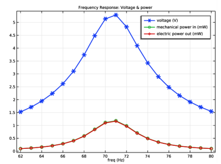
In the Settings window for 1D Plot Group, type Frequency Response: Voltage & Power in the Label text field.
3
Click to expand the Title section. From the Title type list, choose Manual.
4
In the Title text area, type Frequency Response: Voltage & power.
Global 1
1
Right-click Frequency Response: Voltage & Power and choose Global.
2
In the Settings window for Global, locate the y-Axis Data section.
3
4
Click to expand the Coloring and Style section. From the Width list, choose 2.
5
Find the Line markers subsection. From the Marker list, choose Cycle.
6
In the Frequency Response: Voltage & Power toolbar, click  Plot.
Add Study
1
In the Home toolbar, click  Add Study to open the Add Study window.
2
Go to the Add Study window.
3
Find the Studies subsection. In the Select Study tree, select General Studies>Frequency Domain.
4
Click Add Study in the window toolbar.
5
In the Home toolbar, click  Add Study to close the Add Study window.
Study 2
Step 1: Frequency Domain
1
In the Settings window for Frequency Domain, locate the Study Settings section.
2
In the Frequencies text field, type 70.5.
3
Click to expand the Study Extensions section. Select the Auxiliary sweep check box.
4
5
6
In the Model Builder window, click Study 2.
7
In the Settings window for Study, type Load Dependence in the Label text field.
8
Locate the Study Settings section. Clear the Generate default plots check box.
Solution 2 (sol2)
1
In the Study toolbar, click  Show Default Solver.
2
In the Model Builder window, expand the Solution 2 (sol2) node.
3
In the Model Builder window, expand the Load Dependence>Solver Configurations>Solution 2 (sol2)>Stationary Solver 1 node, then click Direct.
4
In the Settings window for Direct, locate the Error section.
5
From the Check error estimate list, choose No.
6
In the Study toolbar, click  Compute.
Results
Load Dependence: Voltage & Power
1
In the Model Builder window, right-click Frequency Response: Voltage & Power and choose Duplicate.
2
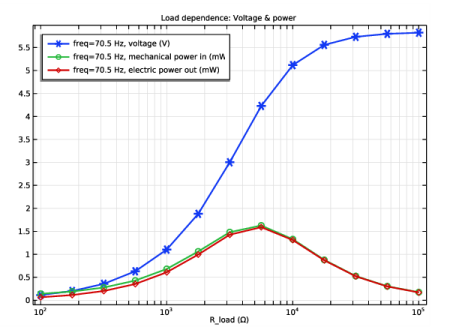
In the Settings window for 1D Plot Group, type Load Dependence: Voltage & Power in the Label text field.
3
Locate the Data section. From the Dataset list, choose Load Dependence/Solution 2 (sol2).
4
Locate the Title section. In the Title text area, type Load dependence: Voltage & power.
5
Locate the Legend section. From the Position list, choose Upper left.
6
Click the  x-Axis Log Scale button in the Graphics toolbar.
7
In the Load Dependence: Voltage & Power toolbar, click  Plot.
Root
From the Home menu, choose Add Study.
Add Study
1
Go to the Add Study window.
2
Find the Studies subsection. In the Select Study tree, select General Studies>Frequency Domain.
3
Click Add Study in the window toolbar.
4
From the Home menu, choose Add Study.
Study 3
Step 1: Frequency Domain
1
In the Settings window for Frequency Domain, locate the Study Settings section.
2
In the Frequencies text field, type 70.5.
3
Locate the Study Extensions section. Select the Auxiliary sweep check box.
4
5
6
In the Model Builder window, expand the Load Dependence: Voltage & Power node, then click Study 3.
7
In the Settings window for Study, type Acceleration Dependence in the Label text field.
8
Locate the Study Settings section. Clear the Generate default plots check box.
Solution 3 (sol3)
1
In the Study toolbar, click  Show Default Solver.
2
In the Model Builder window, expand the Solution 3 (sol3) node.
3
In the Model Builder window, expand the Acceleration Dependence>Solver Configurations>Solution 3 (sol3)>Stationary Solver 1 node, then click Direct.
4
In the Settings window for Direct, locate the Error section.
5
From the Check error estimate list, choose No.
6
In the Study toolbar, click  Compute.
Results
Acceleration Dependence: Voltage & Power
1
In the Model Builder window, right-click Load Dependence: Voltage & Power and choose Duplicate.
2
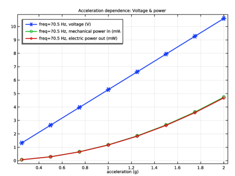
In the Settings window for 1D Plot Group, type Acceleration Dependence: Voltage & Power in the Label text field.
3
Locate the Data section. From the Dataset list, choose Acceleration Dependence/Solution 3 (sol3).
4
Locate the Plot Settings section.
5
Select the x-axis label check box. In the associated text field, type acceleration (g).
6
Locate the Axis section. Clear the x-axis log scale check box.
7
Locate the Title section. In the Title text area, type Acceleration dependence: Voltage & power.
8
In the Acceleration Dependence: Voltage & Power toolbar, click  Plot.