You are viewing the documentation for an older COMSOL version. The latest version is available here.
PDF

Micropump Mechanism1
Micropumps are key components of microfluidic systems with applications ranging from biological fluid handling to microelectronic cooling. This model simulates the mechanism of a valveless micropump, that is designed to be effective at low Reynolds numbers, overcoming hydrodynamic reversibility. Valveless pumps are often preferred in microfluidic systems because they minimize the risk of clogging and are gentle on biological material. The Fluid-Structure Interaction interface is used to solve for the flow of the fluid and the associated deformation of the structure. In addition, the Global ODEs and DAEs interface is used to demonstrate how to perform a time-resolved integration of the total flow throughout the pumping cycle.
Introduction
Many valveless pump designs are ineffective when the system has a low Reynolds number, and consequently are unsuitable for viscous fluids and applications with small length scales or low flow rates. This is largely because without valves it is difficult to achieve sustained flow in a given direction.
The mechanism simulated in this model overcomes this limitation by converting oscillatory fluid motion, induced by a simple reciprocating pumping mechanism, into a net flow in one direction. It is relatively easy to create an oscillatory pumping mechanism in a microfluidic system, for example, a membrane can be vibrated by a piezo oscillator to periodically vary the volume of a microchamber. In this model, an oscillatory flow is fed into a channel containing bendable microflaps. The deformation of the microflaps in response to the motion of the fluid alters the flow and results in a net flow rate in a consistent direction. The passive nature of the flow regulator allows for directional control of the flow without the use of the complicated synchronized actuation mechanisms that would be required in a valve based system.
In this model the Fluid-Structure Interaction Multiphysics interface is used to specify the input oscillatory flow, along with the mechanical properties of the flaps. The deformation of the flaps, and the flow of the fluid, is calculated as a function of time for two full cycles of the pumping mechanism. This allows the physical mechanism responsible for generating the unidirectional flow to be visualized clearly using an animation. As well as visualizing flow rate and direction as a function of time throughout the pumping cycle, integration coupling components are used in conjunction with the Global ODEs and DAEs interface to calculate the net volume pumped from left-to-right as a function of time. This is an example of how the functionality of one COMSOL interface can be enhanced by using a custom equation specified in a mathematics interface, and demonstrates the ease with which user defined equations can be incorporated into COMSOL models.
Model Definition
The model geometry is shown in Figure 1. It consists of a horizontal channel that is 600 μm in length and 100 μm high. A vertical chamber connects to the channel at the midpoint along its length. Two tilted flaps are attached to the bottom of the channel such that they partially obstruct flow along the channel length. They are spaced to be centered on the midpoint of the channel length, and they are both angled at 45 degrees to the horizontal channel edge. Note that this 2D model represents a cross-section through the midpoint of the channel in the out-of-plane direction. An out-of-plane thickness of 10 μm has been used for the purpose of calculating the volume of fluid pumped as a function of time. However, as no edge effects due to walls that are out-of-plane are included, this is equivalent to modeling a 10 μm deep section of a much thicker channel.
Figure 1: The model geometry consists of a horizontal channel and a vertical chamber. Tilted flaps are positioned within the channel, the response of these flaps to the oscillatory fluid motion induced via the labeled boundary results in a net flow from left-to-right.
The physics required for the model is configured within the Fluid-Structure Interaction multiphysics interface. An Inlet boundary feature is applied to the top of the vertical chamber. This specifies the inflow velocity, via a user input expression, to vary sinusoidally in time with a period of 1 s. An Outlet boundary feature is applied to the left and right boundaries of the channel. Two boundary integration coupling components, named intopL() and intopR() for the left and right outlets respectively, are also applied to these outlet boundaries. These are used to compute the flow rate out of each outlet. This is achieved using some user defined variables in the Definitions node within Component 1. The flow rate from each outlet is calculated by integrating the depended variable u_fluid, which is the horizontal component of the fluid velocity, and multiplied by the out-of-plane length scale of 10 μm. The net flow rate out of the channel, UoutNet, is then calculated from the difference between the flow from the left and right outlets, such that positive values correspond to a net flow in the left-to-right direction.
A Global ODEs and DAEs interface is added to compute the integrated net flow as a function of time. This is achieved using a Global Equation which integrates UoutNet with respect to time to obtain Vpump. This step is necessary as UoutNet gives the instantaneous net flow rate as a function in time, however a more useful metric for evaluating a pump is the total volume pumped throughout an entire pumping cycle. Note that the timeint() operator can also be used to visualize the time integration of a variable. However, use of timeint() is not as accurate as directly solving for an integrated quantity, as the timeint() operator only uses the time steps which are saved in the solution but solving directly uses every time step taken by the solver.
The mesh is configured to be tightest around the tilted flaps, in order to resolve the stress within the bending flaps. The mesh is shown in Figure 2.
Figure 2: Initial mesh prior to any structural deformation.
A single time dependent study is performed over a duration of 2 seconds, which corresponds to two full oscillations of the inlet velocity. Some minor amendments to the default solver sequence, described in the step-by-step instructions, are required to ensure reliable results. In particular, the Time Stepping sets the maximum step to 0.01 s. This is needed because the feedback between the flap deformation and the fluid flow can lead to abrupt changes in the flow. The default time stepping setting allows the solver to vary the time step it takes so that larger steps can be taken during times when the solution is not rapidly varying. However, because of the potential for sudden changes to the fluid flow in fluid-structure interaction models it can be helpful to impose a maximum time step to ensure that rapid changes are not missed.
It should be noted that the geometry is parameterized so that the channel dimensions and flap angle can be modified by amending the relevant entry in the Global Parameters table. The average flow rate at the inlet and the fluid properties are also parameterized in the same way. In addition, the effective Reynolds number can be easily changed as the viscosity and average inlet velocity are appropriately scaled by a shared coefficient (the parameter coeff) that is computed from the target Reynolds number (the parameter Re). Note that the parameter Re_check is provided to confirm that the Reynolds number does indeed take the specified value. The model is setup with a Reynolds number of 16, but it is straightforward to verify that the pumping action occurs even for Reynolds numbers significantly less than one.
Results and Discussion
The mechanism by which the flow direction is regulated can be observed in a combined Flow and Stress plot. During the downstroke, when fluid is pushed from the vertical chamber into the channel, the right-hand flap is bent down toward the bottom of the channel whilst the left-hand flap is bend away from the channel bottom. This configuration is shown in Figure 3, which shows the solution at a time of 0.26 s which corresponds to when the velocity flowing into the vertical chamber via the inlet is at its maximum. Due to the asymmetric bending of the flaps, fluid can more easily flow out of the right-hand outlet. During the upstroke, when fluid is drawn from the channel into the vertical chamber, the flaps are bent in the opposite directions. This configuration is shown in Figure 4, which shows the solution at a time of 0.74 s. Now the right hand flap restricts the flow more than the left-hand flap, and the majority of the fluid that is drawn into the vertical chamber is from the left-hand outlet.
The result of this behavior is that there is a net flow rate from left-to-right inside the channel. This has many possible applications in microfluidic systems. For example, this device could be used to deliver fluid from a droplet reservoir connected to the left-hand outlet into a microfluidic pathway connected to the right-hand outlet. Alternately, this device could be used to create a circulating system where a fluid is pumped around a continuous loop to cool a microelectronic system.
Figure 3: Velocity magnitude and velocity field, along with the von Mises stress within the flaps during the pumping down-stroke.
Figure 4: Velocity magnitude and velocity field, along with von Mises stress within the flaps, during the pumping upstroke.
The net volume of fluid that is pumped from left-to-right is shown in Figure 5. As expected, the gradient of the curve, which is the net flow rate, varies sinusoidally with a period equal to the inlet velocity. The maximum gradients occur at intervals of odd multiples of 0.5 s, which correspond with the peaks in the magnitude of the inlet velocity.
Figure 5: Net volume pumped from left-to-right as a function of time.
Application Library path: MEMS_Module/Fluid-Structure_Interaction/micropump_mechanism
Modeling Instructions
From the File menu, choose New.
New
In the New window, click  Model Wizard.
Model Wizard
1
In the Model Wizard window, click  2D.
2
In the Select Physics tree, select Fluid Flow>Fluid-Structure Interaction>Fluid-Solid Interaction.
3
Click Add.
4
Click  Study.
5
In the Select Study tree, select General Studies>Time Dependent.
6
Geometry 1
Add some parameters which will be used to control the fluid properties and device geometry.
Global Definitions
Parameters 1
1
In the Model Builder window, under Global Definitions click Parameters 1.
2
In the Settings window for Parameters, locate the Parameters section.
3
Next create the geometry for the device.
Geometry 1
1
In the Model Builder window, under Component 1 (comp1) click Geometry 1.
2
In the Settings window for Geometry, locate the Units section.
3
From the Length unit list, choose µm.
Rectangle 1 (r1)
1
In the Geometry toolbar, click  Rectangle.
2
In the Settings window for Rectangle, locate the Size and Shape section.
3
In the Width text field, type L.
4
In the Height text field, type H.
5
Locate the Position section. In the x text field, type -L/2.
Rectangle 2 (r2)
1
In the Geometry toolbar, click  Rectangle.
2
In the Settings window for Rectangle, locate the Size and Shape section.
3
In the Width text field, type 2*rp.
4
In the Height text field, type 2*hp.
5
Locate the Position section. From the Base list, choose Center.
6
In the x text field, type x0-hp*sin(beta)/2.
7
Locate the Rotation Angle section. In the Rotation text field, type -beta.
Copy 1 (copy1)
1
In the Geometry toolbar, click  Transforms and choose Copy.
2
Intersection 1 (int1)
1
In the Geometry toolbar, click  Booleans and Partitions and choose Intersection.
2
Select the objects r1 and r2 only.
3
In the Settings window for Intersection, locate the Intersection section.
4
Clear the Keep interior boundaries check box.
Fillet 1 (fil1)
1
In the Geometry toolbar, click  Fillet.
2
On the object int1, select Points 3 and 4 only.
It might be easier to select the correct points by using the Selection List window. To open this window, in the Home toolbar click Windows and choose Selection List. (If you are running the cross-platform desktop, you find Windows in the main menu.)
3
In the Settings window for Fillet, locate the Radius section.
4
In the Radius text field, type rp.
Copy 2 (copy2)
1
In the Geometry toolbar, click  Transforms and choose Copy.
2
3
In the Settings window for Copy, locate the Displacement section.
4
In the x text field, type -2*x0.
Rectangle 3 (r3)
1
In the Geometry toolbar, click  Rectangle.
2
In the Settings window for Rectangle, locate the Size and Shape section.
3
In the Width text field, type 0.8*H.
4
In the Height text field, type H.
5
Locate the Position section. In the x text field, type -0.4*H.
6
In the y text field, type H.
7
Click  Build All Objects.
Add two nonlocal integration couplings, one to the boundary which forms the left outlet and one to the boundary which forms the right outlet. These couplings will be used to calculate the flow rate out of each outlet.
Definitions
Integration 1 (intop1)
1
In the Definitions toolbar, click  Nonlocal Couplings and choose Integration.
2
In the Settings window for Integration, type intopL in the Operator name text field.
3
Locate the Source Selection section. From the Geometric entity level list, choose Boundary.
4
Integration 2 (intop2)
1
In the Definitions toolbar, click  Nonlocal Couplings and choose Integration.
2
In the Settings window for Integration, type intopR in the Operator name text field.
3
Locate the Source Selection section. From the Geometric entity level list, choose Boundary.
4
Create some variables to calculate the net flow rate in the channel. The first two variables calculate the average flow rate out of each outlet by performing an average over u_fluid , which is the horizontal component of the fluid flow. Note the sign convention, that assigns positive values to left-right flow and negative values to right-left flow. The third variable calculates the difference between the average flow rate out of each outlet, positive values correspond to a net flow from left to right.
Variables 1
1
In the Model Builder window, right-click Definitions and choose Variables.
2
In the Settings window for Variables, locate the Variables section.
3
In order to integrate the average net flow rate over time to calculate the volume of fluid that is pumped, add a Global ODE and DAEs physics interface to the model.
Add Physics
1
In the Home toolbar, click  Add Physics to open the Add Physics window.
2
Go to the Add Physics window.
3
In the tree, select Mathematics>ODE and DAE Interfaces>Global ODEs and DAEs (ge).
4
Click Add to Component 1 in the window toolbar.
5
In the Home toolbar, click  Add Physics to close the Add Physics window.
Global ODEs and DAEs (ge)
Global Equations 1
1
In the Model Builder window, under Component 1 (comp1)>Global ODEs and DAEs (ge) click Global Equations 1.
2
In the Settings window for Global Equations, locate the Global Equations section.
3
4
Locate the Units section. Click  Define Dependent Variable Unit.
5
In the Dependent variable quantity table, enter the following settings:
6
Click  Define Source Term Unit.
7
In the Source term quantity table, enter the following settings:
Configure the Fluid-Structure Interaction physics interface.
Moving Mesh
Deforming Domain 1
1
In the Model Builder window, under Component 1 (comp1)>Moving Mesh click Deforming Domain 1.
2
In the Settings window for Deforming Domain, locate the Smoothing section.
3
In the C2 text field, type 100.
4
Component 1 (comp1)
Fixed Boundary 1
1
In the Definitions toolbar, click  Moving Mesh and choose Boundaries>Fixed Boundary.
2
Prescribed Normal Mesh Displacement 1
1
In the Definitions toolbar, click  Moving Mesh and choose Boundaries>Prescribed Normal Mesh Displacement.
2
Laminar Flow (spf)
1
In the Model Builder window, under Component 1 (comp1) click Laminar Flow (spf).
2
Inlet 1
1
In the Physics toolbar, click  Boundaries and choose Inlet.
2
3
In the Settings window for Inlet, locate the Velocity section.
4
In the U0 text field, type U*6*s*(1-s)*sin(2*pi*t/(1[s])).
Outlet 1
1
In the Physics toolbar, click  Boundaries and choose Outlet.
2
3
In the Settings window for Outlet, locate the Pressure Conditions section.
4
Clear the Suppress backflow check box.
Solid Mechanics (solid)
1
In the Model Builder window, under Component 1 (comp1) click Solid Mechanics (solid).
2
Linear Elastic Material 1
1
In the Model Builder window, under Component 1 (comp1)>Solid Mechanics (solid) click Linear Elastic Material 1.
2
In the Settings window for Linear Elastic Material, locate the Linear Elastic Material section.
3
From the Use mixed formulation list, choose Pressure formulation.
Fixed Constraint 1
1
In the Physics toolbar, click  Boundaries and choose Fixed Constraint.
2
With the physics interfaces configured, add materials to the geometry domains. In this case, it was beneficial to wait until all the physics settings were configured before adding materials, as COMSOL automatically adjusts which materials properties are needed depending on the physics assigned to each domain.
Materials
Fluid
1
In the Model Builder window, under Component 1 (comp1) right-click Materials and choose Blank Material.
2
In the Settings window for Material, type Fluid in the Label text field.
Solid
1
Right-click Materials and choose Blank Material.
2
In the Settings window for Material, type Solid in the Label text field.
3
Fluid (mat1)
1
In the Model Builder window, click Fluid (mat1).
2
In the Settings window for Material, locate the Material Contents section.
3
Solid (mat2)
1
In the Model Builder window, click Solid (mat2).
2
In the Settings window for Material, locate the Material Contents section.
3
Configure the mesh.
Mesh 1
Free Triangular 1
1
In the Mesh toolbar, click  Free Triangular.
2
In the Settings window for Free Triangular, locate the Domain Selection section.
3
From the Geometric entity level list, choose Entire geometry.
Size
1
In the Model Builder window, click Size.
2
In the Settings window for Size, locate the Element Size section.
3
Click the Custom button.
4
Locate the Element Size Parameters section. In the Maximum element size text field, type 10.
5
In the Minimum element size text field, type 1.4.
6
In the Maximum element growth rate text field, type 1.4.
7
In the Curvature factor text field, type 0.6.
8
In the Resolution of narrow regions text field, type 0.7.
Size 1
1
In the Model Builder window, right-click Mesh 1 and choose Size.
2
Right-click Size 1 and choose Move Up.
3
In the Settings window for Size, locate the Geometric Entity Selection section.
4
From the Geometric entity level list, choose Domain.
5
6
Locate the Element Size section. Click the Custom button.
7
Locate the Element Size Parameters section.
8
Select the Maximum element size check box. In the associated text field, type 2.
9
Select the Minimum element size check box. In the associated text field, type 1.5.
10
In the Model Builder window, right-click Mesh 1 and choose Build All.
Configure the study.
Set the time steps and range for the study.
Study 1
Step 1: Time Dependent
1
In the Model Builder window, under Study 1 click Step 1: Time Dependent.
2
In the Settings window for Time Dependent, locate the Study Settings section.
3
In the Output times text field, type range(0,0.02,2).
4
In the Home toolbar, click  Compute.
Results
Velocity (spf)
Modify the default Velocity plot group to show the von Mises stress within the flexible rods, as well as the velocity magnitude of the fluid within the channel. Add an Arrow Surface plot of the fluid velocity. An animation of the data series allows the action of the pump to be visualized.
Study 1/Solution 1 (2) (sol1)
1
In the Model Builder window, expand the Results>Datasets node.
2
Right-click Results>Datasets>Study 1/Solution 1 (sol1) and choose Duplicate.
With this new dataset you refer to the spatial frame which allows to visualize the data on the deformed configuration.
Flow and Stress
1
In the Model Builder window, under Results click Velocity (spf).
2
In the Settings window for 2D Plot Group, type Flow and Stress in the Label text field.
3
Locate the Data section. From the Dataset list, choose Study 1/Solution 1 (2) (sol1).
Surface 2
1
Right-click Flow and Stress and choose Surface.
2
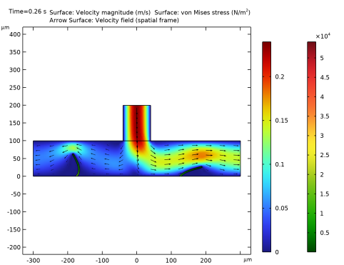
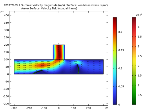
In the Settings window for Surface, click Replace Expression in the upper-right corner of the Expression section. From the menu, choose Component 1 (comp1)>Solid Mechanics>Stress>solid.mises - von Mises stress - N/m².
3
Locate the Coloring and Style section. Click  Change Color Table.
4
In the Color Table dialog box, select Traffic>Traffic in the tree.
5
Arrow Surface 1
1
Right-click Flow and Stress and choose Arrow Surface.
2
In the Settings window for Arrow Surface, locate the Coloring and Style section.
3
From the Arrow length list, choose Logarithmic.
4
From the Color list, choose Black.
5
In the Flow and Stress toolbar, click  Plot.
Animation 1
1
In the Results toolbar, click  Animation and choose File.
2
In the Settings window for Animation, locate the Target section.
3
From the Target list, choose Player.
4
Locate the Frames section. From the Frame selection list, choose All.
5
Click the  Play button in the Graphics toolbar.
The animation demonstrates how the passive motion of the rods as they react to the fluid results in a net flow of fluid from left-to-right. During the "downstroke", when fluid flows from the inlet down into the channel, the right rod bends toward the bottom of the channel whilst the left rod bend away from the bottom. This restricts the flow toward the left-hand outlet, relative to the right-hand outlet. During the "upstroke", where fluid flows from the channel up toward the inlet, the rods bend in the opposite directions. Now the inward flow from the right-hand outlet toward the center of the channel is restricted. This results in a net flow from left-to-right, where fluid is drawn in from the left-hand outlet and pushed out of the right-hand outlet.
The 1D plot group, which plots Vpump from the Global ODEs and DAEs interface, confirms that there is indeed a net flow from left-to-right as expected.
Net Volume Pumped Left-to-Right
1
In the Model Builder window, under Results click 1D Plot Group 4.
2
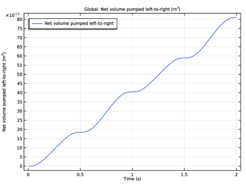
In the Settings window for 1D Plot Group, type Net Volume Pumped Left-to-Right in the Label text field.
3
Locate the Legend section. From the Position list, choose Upper left.
 

1
This model is courtesy of Matthew J. Hancock and Stuart Brown of Veryst Engineering, LLC.