You are viewing the documentation for an older COMSOL version. The latest version is available here.
PDF

Electrostrictive Disc
Introduction
The electrostrictive effect describes the electric field-induced strain within a material. It is particularly important for a class of materials known as relaxor ferroelectrics. Such materials are composed of ferroelectric domains that are randomly oriented in the absence of an electric field in the material. In the presence of an electric field, these domains rotate, thereby producing strain in the material. The material extends in the direction of electric field and contracts in the direction perpendicular to the field. On applying an electric field in the reverse direction, the ferroelectric domains orient in the same direction as the field, but the material still elongates and hence electrostriction produces unidirectional strain. To produce a bidirectional strain the material can be subjected to an AC electric field superimposed on a DC bias. At very large electric fields, the electrostrictive strain saturates as all ferroelectric domains in the material align along the direction of the electric field. One of the popular electrostrictive ceramic materials is PMN-PT (lead magnesium niobate-lead titanate), which is often used with some dopant, for example, with barium titanate (BT).
Relaxor ferroelectrics have very high dielectric constants, consequently large polarizations are generated by these materials as a result of an applied electric field. There is very little hysteresis in the response of these materials to electric fields, which makes them attractive for micropositioning devices. A consequence of the absence of hysteresis is that there is negligible self-heating (dielectric heating) in dynamic applications and these materials are therefore used in sonars and ultrasonic motors. Unlike piezoelectric materials, they do not need to be poled. Since there is no residual polarization in the absence of an electric field, a mechanical stress does not change the electric field in the material. Hence these materials are in general not used in sensors.
In this tutorial, you learn how to model isotropic ferroelectroelastic materials using COMSOL’s Ferroelectroelasticity interface. This application requires either the MEMS Module or the AC/DC Module and Structural Mechanics Module.
Model Definition
This tutorial shows how to model an electrostrictive cylindrical disc surrounded by air. The geometry is axisymmetric, and consequently 2D axisymmetry is used. The geometry is shown in Figure 1.
The upper end of the disc is at electrical ground whereas the voltage at the lower end is quasi-statically varied from zero to +103 V volts by using the continuation parameter approach in the study settings.
Because of the symmetry, it is sufficient to model only the upper half of the disc using the symmetry boundary conditions.
Figure 1: Axisymmetric model geometry. The ferroelectroelastic disc is in the center of the geometry, the remain of the domain shows the surrounding air.
Electrostriction for a material of arbitrary symmetry can be represented as the following additive contribution to the strain:
(1)
which is quadratic in polarization P. However, for isotropic materials, the fourth order tensor Q has only two independent components, which are usually denoted as Q11 and Q12.
For ferroelectroelastic materials, the polarization vector is nonlinear function of the electric field and possible stress in the material. One possible choice of the polarization shape is hyperbolic tangent (Ref. 1):
(2)
where Ps is the saturation polarization, a is a material parameter called the domain wall density, and the effective electric field is given by
(3)
where E is the applied electric field, and the mechanics stress is computed assuming mechanically linear material as
(4)
where the strain is computed from the mechanical displacement
Again, for isotropic materials, the fourth-order elasticity tensor C has only two independent components. Most common choice to represent those are by specifying the Young’s modulus EYM and Poisson’s ratio ν for the material.
The effective tangential piezoelectric coupling coefficients can be computed as
where ε0,vac is the electric permittivity of free space, and
is the tangent electric susceptibility. An important observation from the above formula is that the piezoelectric coefficients should reach their maximum (or minimum) at certain strength of the applied bias field. This is because P is zero at zero applied field, while χ tends to zero at large applied field magnitudes because of saturation. The piezoelectric coupling tensor d is a third-order tensor. Due to the symmetry, it can be conventionally represented by a 3-by-6 matrix dET with only few nonzero components.
The following material data has been measured (Ref. 1) for a PMT-PT-BT relaxor-ferroelectric material that presents a ternary mixture of lead magnesium niobate with 7.7% lead titanate and 2.5% barium titanate:
EYM
105 GPa
ν
ρ
Ps
Q11
Q12
The air domain is modeled with an additional layer on its periphery.
The voltage applied at the disk lower boundary is gradually varying from zero to 4 kV. The upper boundary of the disc is electrically grounded, and it can be loaded mechanically to study the inverse electrostrictive effect. Three cases are analyzed: one without mechanical loading and two others using a vertical boundary load of 40 GPa and 80 GPa, respectively.
Results and Discussion
Figure 2 shows the distribution of the electric potential in the material and in air around it. In Figure 3, the displacement magnitude is visualized in 3D in case of no mechanical loading.
Figure 2: Surface plot of electric potential distribution in the electrostrictive material and surrounding air domain for a 4 kV applied voltage.
.
Figure 3: Surface plot of the mechanical displacement magnitude.
Figure 4 shows a plot of the z-component of polarization plotted against the Z-component of the electric field at the center of the disc. Figure 5 shows a similar plot of the ZZ-component of electrostrictive strain at the same position. A series of both negative and positive voltages applied on the top surface of the disc lead to a change in the sign and hence the direction of the electric field. However, the strain and displacement is always unidirectional.
Figure 4: Axial polarization vs. axial electric field at the center of the disc.
Figure 5: Axial electrostrictive strain vs. axial electric field at the center of the disc.
Finally, Figure 6 shows the effective tangent piezoelectric coefficients computed at a given value of the applied electric field.
Figure 6: Tangent piezoelectric coupling coefficients vs. axial electric field at the center of the disc.
Reference
1. C.L. Horn and N. Shankar, “A finite element method for electrostrictive ceramic devices,” Int. J. Solids Structures, vol. 33, pp. 1757–1779, 1995.
Application Library path: MEMS_Module/Actuators/electrostrictive_disc
Modeling Instructions
From the File menu, choose New.
New
In the New window, click  Model Wizard.
Model Wizard
1
In the Model Wizard window, click  2D Axisymmetric.
2
In the Select Physics tree, select Structural Mechanics>Electromagnetics-Structure Interaction>Ferroelectroelasticity.
3
Click Add.
4
Click  Study.
5
In the Select Study tree, select General Studies>Stationary.
6
Global Definitions
Create parameters to define the geometry, material properties, and applied loads.
Parameters 1
1
In the Model Builder window, under Global Definitions click Parameters 1.
2
In the Settings window for Parameters, locate the Parameters section.
3
Definitions
Variables 1
1
In the Model Builder window, under Component 1 (comp1) right-click Definitions and choose Variables.
2
In the Settings window for Variables, locate the Variables section.
3
This variation of the potential with respect to the parameter at one of the disc boundaries will cause the electric field within the material to gradually change between -Vmax and Vmax.
Geometry 1
Rectangle 1 (r1)
1
In the Geometry toolbar, click  Rectangle.
2
In the Settings window for Rectangle, locate the Size and Shape section.
3
In the Width text field, type R0.
4
In the Height text field, type H0/2.
Rectangle 2 (r2)
1
Right-click Rectangle 1 (r1) and choose Duplicate.
2
In the Settings window for Rectangle, locate the Size and Shape section.
3
In the Width text field, type 3*R0.
4
In the Height text field, type 5*H0/2.
5
Click  Build All Objects.
Solid Mechanics (solid)
1
In the Model Builder window, under Component 1 (comp1) click Solid Mechanics (solid).
2
Symmetry Plane 1
1
In the Physics toolbar, click  Boundaries and choose Symmetry Plane.
2
Boundary Load 1
1
In the Physics toolbar, click  Boundaries and choose Boundary Load.
2
3
In the Settings window for Boundary Load, locate the Force section.
4
Specify the FA vector as
Electrostatics (es)
In the Model Builder window, under Component 1 (comp1) click Electrostatics (es).
Ground 1
1
In the Physics toolbar, click  Boundaries and choose Ground.
2
Electric Potential 1
1
In the Physics toolbar, click  Boundaries and choose Electric Potential.
2
Because of the symmetry, the voltage at the horizontal symmetry plane equals to a half of that applied at the bottom surface.
3
In the Settings window for Electric Potential, locate the Electric Potential section.
4
In the V0 text field, type V0/2.
Charge Conservation, Ferroelectric 1
1
In the Model Builder window, click Charge Conservation, Ferroelectric 1.
2
3
In the Settings window for Charge Conservation, Ferroelectric, locate the Ferroelectric Material Properties section.
4
Find the Anhysteretic polarization subsection. From the Anhysteretic polarization shape list, choose Hyperbolic tangent.
5
Find the Effective electric field subsection. From the α list, choose User defined. In the associated text field, type 0.
Multiphysics
Electrostriction 1 (efe1)
1
In the Model Builder window, under Component 1 (comp1)>Multiphysics click Electrostriction 1 (efe1).
2
In the Settings window for Electrostriction, locate the Coupling Type section.
3
From the list, choose Fully coupled.
4
Locate the Electrostriction section. In the Q11 text field, type Q11.
5
In the Q12 text field, type Q12.
Add Material
1
In the Home toolbar, click  Add Material to open the Add Material window.
2
Go to the Add Material window.
3
4
Right-click and choose Add to Component 1 (comp1).
5
In the Home toolbar, click  Add Material to close the Add Material window.
Materials
PMT-PT-BT
1
In the Model Builder window, under Component 1 (comp1) right-click Materials and choose Blank Material.
2
In the Settings window for Material, type PMT-PT-BT in the Label text field.
3
4
Locate the Material Contents section. In the table, enter the following settings:
Mesh 1
Mapped 1
1
In the Mesh toolbar, click  Mapped.
2
In the Settings window for Mapped, locate the Domain Selection section.
3
From the Geometric entity level list, choose Domain.
4
Distribution 1
1
Right-click Mapped 1 and choose Distribution.
2
3
In the Settings window for Distribution, locate the Distribution section.
4
In the Number of elements text field, type 4.
Distribution 2
1
In the Model Builder window, right-click Mapped 1 and choose Distribution.
2
3
In the Settings window for Distribution, locate the Distribution section.
4
In the Number of elements text field, type 16.
Size
1
In the Model Builder window, under Component 1 (comp1)>Mesh 1 click Size.
2
In the Settings window for Size, locate the Element Size section.
3
From the Predefined list, choose Finer.
Free Triangular 1
1
In the Mesh toolbar, click  Free Triangular.
2
In the Settings window for Free Triangular, click  Build All.
Study 1
Change the study settings to sweep over applied voltage.
Step 1: Stationary
1
In the Model Builder window, under Study 1 click Step 1: Stationary.
2
In the Settings window for Stationary, click to expand the Study Extensions section.
3
Select the Auxiliary sweep check box.
4
5
Parametric Sweep
1
In the Study toolbar, click  Parametric Sweep.
2
In the Settings window for Parametric Sweep, locate the Study Settings section.
3
4
5
In the Study toolbar, click  Compute.
Results
Surface 1
The first and second default plots show the stress distribution in the disc, which is almost uniform.
1
In the Model Builder window, expand the Results>Stress (solid) node, then click Surface 1.
2
In the Settings window for Surface, locate the Expression section.
3
From the Unit list, choose MPa.
4
In the Stress (solid) toolbar, click  Plot.
Displacement, 3D (solid)
1
In the Model Builder window, under Results click Stress, 3D (solid).
2
In the Settings window for 3D Plot Group, locate the Data section.
3
From the Parameter value (F0 (MPa)) list, choose 0.
4
From the Parameter value (t (s)) list, choose 0.25.
5
In the Label text field, type Displacement, 3D (solid).
Surface 1
1
In the Model Builder window, expand the Displacement, 3D (solid) node, then click Surface 1.
2
In the Settings window for Surface, locate the Expression section.
3
In the Expression text field, type solid.disp.
4
From the Unit list, choose µm.
5
In the Displacement, 3D (solid) toolbar, click  Plot.
Electric Potential (es)
The fourth default plots shows the electric potential distribution.
1
In the Model Builder window, under Results click Electric Potential (es).
2
In the Settings window for 2D Plot Group, locate the Data section.
3
From the Parameter value (t (s)) list, choose 0.25.
4
In the Electric Potential (es) toolbar, click  Plot.
Plot the electrostrictive strain and polarization in the middle of the disc versus the applied field.
Electrostrictive Strain
1
In the Home toolbar, click  Add Plot Group and choose 1D Plot Group.
2
In the Settings window for 1D Plot Group, type Electrostrictive Strain in the Label text field.
3
Locate the Data section. From the Dataset list, choose Study 1/Parametric Solutions 1 (sol2).
4
Click to expand the Title section. From the Title type list, choose Manual.
5
In the Title text area, type Axial strain vs. Axial electric field.
6
Locate the Legend section. From the Position list, choose Upper middle.
Point Graph 1
1
Right-click Electrostrictive Strain and choose Point Graph.
2
3
In the Settings window for Point Graph, locate the y-Axis Data section.
4
In the Expression text field, type efe1.emZZ.
5
From the Unit list, choose ppm.
6
Locate the x-Axis Data section. From the Parameter list, choose Expression.
7
In the Expression text field, type es.EZ.
8
From the Unit list, choose MV/m.
9
Click to expand the Legends section. Select the Show legends check box.
10
Find the Include subsection. Clear the Point check box.
11
In the Electrostrictive Strain toolbar, click  Plot.
Polarization
1
In the Model Builder window, right-click Electrostrictive Strain and choose Duplicate.
2
In the Settings window for 1D Plot Group, type Polarization in the Label text field.
3
Locate the Title section. In the Title text area, type Axial polarization vs. Axial electric field.
4
Locate the Legend section. From the Position list, choose Lower right.
Point Graph 1
1
In the Model Builder window, expand the Polarization node, then click Point Graph 1.
2
In the Settings window for Point Graph, locate the y-Axis Data section.
3
In the Expression text field, type es.PZ.
4
In the Polarization toolbar, click  Plot.
Finally, plot the tangent piezoelectric coupling coefficients.
Tangent Piezoelectric Coupling Coefficients
1
In the Model Builder window, right-click Polarization and choose Duplicate.
2
In the Settings window for 1D Plot Group, locate the Data section.
3
From the Parameter selection (F0) list, choose First.
4
In the Label text field, type Tangent Piezoelectric Coupling Coefficients.
5
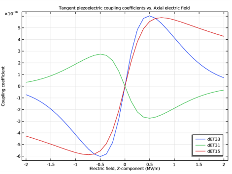
Locate the Title section. In the Title text area, type Tangent piezoelectric coupling coefficients vs. Axial electric field.
6
Locate the Plot Settings section.
7
Select the y-axis label check box. In the associated text field, type Coupling coefficient.
8
Locate the Grid section. Select the Manual spacing check box.
9
In the x spacing text field, type 0.5.
10
In the y spacing text field, type 1e-10.
Point Graph 1
1
In the Model Builder window, expand the Tangent Piezoelectric Coupling Coefficients node, then click Point Graph 1.
2
In the Settings window for Point Graph, locate the y-Axis Data section.
3
In the Expression text field, type efe1.dET33.
4
Locate the Legends section. From the Legends list, choose Manual.
5
Point Graph 2
1
Right-click Results>Tangent Piezoelectric Coupling Coefficients>Point Graph 1 and choose Duplicate.
2
In the Settings window for Point Graph, locate the y-Axis Data section.
3
In the Expression text field, type efe1.dET31.
4
Locate the Legends section. In the table, enter the following settings:
Point Graph 3
1
Right-click Point Graph 2 and choose Duplicate.
2
In the Settings window for Point Graph, locate the y-Axis Data section.
3
In the Expression text field, type efe1.dET15.
4
Locate the Legends section. In the table, enter the following settings:
5
In the Tangent Piezoelectric Coupling Coefficients toolbar, click  Plot.