|
|
|


|
1
|
|
2
|
|
3
|
Click Add.
|
|
4
|
Click
|
|
5
|
|
6
|
Click
|
|
1
|
|
2
|
|
3
|
|
1
|
|
2
|
|
3
|
Locate the Parameters section. In the table, enter the following settings:
|
|
1
|
|
2
|
|
3
|
Locate the Parameters section. In the table, enter the following settings:
|
|
1
|
|
2
|
|
1
|
|
2
|
|
3
|
|
4
|
|
5
|
|
6
|
|
7
|
Locate the Selections of Resulting Entities section. Find the Cumulative selection subsection. Click New.
|
|
8
|
|
9
|
Click OK.
|
|
1
|
|
2
|
In the Settings window for Rectangle, type Rectangle 2 - Footprint of sense electrode in the Label text field.
|
|
3
|
|
4
|
|
1
|
|
2
|
|
3
|
|
4
|
|
5
|
Locate the Selections of Resulting Entities section. Find the Cumulative selection subsection. From the Contribute to list, choose Mass.
|
|
1
|
|
2
|
|
3
|
|
4
|
|
5
|
|
6
|
|
7
|
|
8
|
Locate the Selections of Resulting Entities section. Find the Cumulative selection subsection. Click New.
|
|
9
|
|
10
|
Click OK.
|
|
1
|
|
2
|
|
3
|
|
4
|
|
5
|
|
6
|
|
7
|
|
1
|
|
2
|
|
3
|
|
4
|
|
1
|
|
2
|
|
3
|
|
4
|
|
1
|
|
2
|
|
3
|
Locate the Distances section. In the table, enter the following settings:
|
|
4
|
Locate the Selections of Resulting Entities section. Select the Resulting objects selection check box.
|
|
5
|
|
6
|
|
1
|
|
2
|
|
1
|
|
2
|
|
3
|
|
4
|
|
5
|
|
6
|
|
7
|
|
8
|
Locate the Selections of Resulting Entities section. Find the Cumulative selection subsection. Click New.
|
|
9
|
|
10
|
Click OK.
|
|
1
|
|
2
|
|
3
|
Locate the Position section. In the xw text field, type y_spring_l/2+w_mass/2+w_stator_base/2+2*l_rotor-rotor_stator_overlap.
|
|
4
|
|
1
|
|
2
|
|
3
|
|
4
|
|
1
|
In the Model Builder window, under Component 1 (comp1)>Geometry 1>Work Plane 2 - Anchors (wp2)>Plane Geometry right-click Rectangle 2 - Stator Anchor (r2) and choose Duplicate.
|
|
2
|
|
3
|
|
1
|
|
2
|
|
3
|
|
4
|
|
5
|
|
6
|
|
1
|
|
2
|
|
3
|
Locate the Distances section. In the table, enter the following settings:
|
|
4
|
|
5
|
Locate the Selections of Resulting Entities section. Select the Resulting objects selection check box.
|
|
6
|
|
7
|
|
1
|
|
2
|
|
1
|
|
2
|
|
3
|
|
4
|
|
5
|
|
6
|
|
7
|
Locate the Selections of Resulting Entities section. Find the Cumulative selection subsection. Click New.
|
|
8
|
|
9
|
Click OK.
|
|
1
|
|
2
|
|
3
|
|
4
|
|
5
|
|
6
|
|
7
|
|
8
|
Locate the Selections of Resulting Entities section. Find the Cumulative selection subsection. Click New.
|
|
9
|
|
10
|
Click OK.
|
|
1
|
|
2
|
|
3
|
|
4
|
|
5
|
|
6
|
|
7
|
Locate the Selections of Resulting Entities section. Find the Cumulative selection subsection. From the Contribute to list, choose Mirror XY.
|
|
1
|
|
2
|
|
3
|
|
4
|
|
5
|
|
6
|
|
1
|
|
2
|
|
3
|
|
4
|
|
1
|
|
2
|
|
3
|
|
4
|
|
5
|
|
6
|
|
1
|
|
2
|
|
3
|
Locate the Distances section. In the table, enter the following settings:
|
|
4
|
Locate the Selections of Resulting Entities section. Select the Resulting objects selection check box.
|
|
5
|
|
6
|
|
1
|
|
2
|
|
1
|
|
2
|
|
3
|
|
4
|
|
5
|
|
6
|
|
7
|
|
8
|
Locate the Selections of Resulting Entities section. Find the Cumulative selection subsection. Click New.
|
|
9
|
|
10
|
Click OK.
|
|
1
|
|
2
|
|
3
|
|
4
|
|
5
|
|
6
|
|
1
|
|
2
|
|
3
|
|
4
|
|
5
|
|
1
|
|
2
|
|
3
|
|
4
|
|
1
|
|
2
|
|
3
|
Locate the Distances section. In the table, enter the following settings:
|
|
4
|
Locate the Selections of Resulting Entities section. Select the Resulting objects selection check box.
|
|
5
|
|
6
|
|
1
|
|
2
|
|
1
|
|
2
|
|
3
|
|
4
|
|
5
|
|
6
|
|
7
|
|
8
|
Locate the Selections of Resulting Entities section. Find the Cumulative selection subsection. Click New.
|
|
9
|
|
10
|
Click OK.
|
|
1
|
|
2
|
|
3
|
|
4
|
|
5
|
|
6
|
|
1
|
|
2
|
|
3
|
|
4
|
|
5
|
|
6
|
|
7
|
Locate the Selections of Resulting Entities section. Find the Cumulative selection subsection. Click New.
|
|
8
|
|
9
|
Click OK.
|
|
1
|
|
2
|
|
3
|
|
4
|
|
5
|
|
1
|
|
2
|
|
3
|
|
4
|
|
1
|
|
2
|
|
3
|
|
4
|
|
1
|
|
2
|
|
3
|
Locate the Size and Shape section. In the Width text field, type 2*(y_spring_l/2-l_mass/2-l_rotor-(l_rotor-rotor_stator_overlap)).
|
|
4
|
|
5
|
|
6
|
Locate the Selections of Resulting Entities section. Find the Cumulative selection subsection. From the Contribute to list, choose Stator Base.
|
|
1
|
|
2
|
|
3
|
Locate the Distances section. In the table, enter the following settings:
|
|
4
|
Locate the Selections of Resulting Entities section. Select the Resulting objects selection check box.
|
|
5
|
|
6
|
|
1
|
|
2
|
In the Settings window for Work Plane, type Work Plane 6 - Sense Electrodes in the Label text field.
|
|
3
|
|
4
|
Locate the Selections of Resulting Entities section. Select the Resulting objects selection check box.
|
|
1
|
|
2
|
|
3
|
|
4
|
|
5
|
|
6
|
|
7
|
Locate the Selections of Resulting Entities section. Find the Cumulative selection subsection. Click New.
|
|
8
|
|
9
|
Click OK.
|
|
1
|
|
2
|
|
3
|
|
4
|
|
5
|
Locate the Selections of Resulting Entities section. Find the Cumulative selection subsection. From the Contribute to list, choose Sense electrode.
|
|
1
|
|
2
|
|
3
|
|
4
|
|
1
|
|
2
|
|
3
|
|
1
|
|
2
|
|
3
|
|
4
|
|
5
|
Click OK.
|
|
1
|
|
2
|
|
3
|
|
4
|
|
5
|
|
6
|
|
7
|
|
1
|
|
2
|
|
3
|
|
4
|
|
1
|
|
2
|
|
3
|
|
4
|
|
1
|
|
2
|
In the Settings window for Intersection, type Intersection 1 - Lower Electrode in the Label text field.
|
|
3
|
|
4
|
|
5
|
|
6
|
Click OK.
|
|
7
|
|
8
|
|
9
|
|
10
|
Click OK.
|
|
1
|
|
2
|
|
3
|
|
4
|
Locate the Box Limits section. In the x minimum text field, type y_spring_l/2+w_mass/2+l_rotor/2-delta.
|
|
5
|
|
6
|
|
7
|
|
8
|
|
9
|
|
1
|
|
2
|
|
3
|
Locate the Box Limits section. In the x minimum text field, type -(y_spring_l/2+w_mass/2+l_rotor/2)-delta.
|
|
4
|
|
1
|
|
2
|
|
3
|
Locate the Box Limits section. In the x minimum text field, type y_spring_l/2-w_mass/2-l_rotor/2 -delta.
|
|
4
|
|
1
|
|
2
|
|
3
|
Locate the Box Limits section. In the x minimum text field, type -(y_spring_l/2-w_mass/2-l_rotor/2)-delta.
|
|
4
|
|
1
|
|
2
|
|
3
|
|
4
|
|
5
|
In the Add dialog box, in the Selections to add list, choose Box 4 - Comb vertical walls 1, Box 5 - Comb vertical walls 2, Box 6 - Comb vertical walls 3, and Box 7 - Comb vertical walls 4.
|
|
6
|
Click OK.
|
|
1
|
|
2
|
In the Settings window for Intersection, type Intersection 2 - Stator Vertical Walls in the Label text field.
|
|
3
|
|
4
|
|
5
|
In the Add dialog box, in the Selections to intersect list, choose Union 1 - Comb Vertical Walls and Extrude 5 - Stators.
|
|
6
|
Click OK.
|
|
1
|
|
2
|
|
3
|
|
4
|
Locate the Box Limits section. In the x minimum text field, type y_spring_l/2+w_mass/2+l_rotor-delta.
|
|
5
|
|
1
|
|
2
|
|
3
|
Locate the Box Limits section. In the x minimum text field, type -(y_spring_l/2+w_mass/2+l_rotor)-delta.
|
|
4
|
|
1
|
|
2
|
|
3
|
Locate the Box Limits section. In the x minimum text field, type y_spring_l/2-w_mass/2-l_rotor -delta.
|
|
4
|
|
1
|
|
2
|
|
3
|
Locate the Box Limits section. In the x minimum text field, type -(y_spring_l/2-w_mass/2-l_rotor)-delta.
|
|
4
|
|
1
|
|
2
|
|
3
|
|
4
|
|
5
|
In the Add dialog box, in the Selections to add list, choose Box 8 - Rotor tip edge 1 and Box 11 - Rotor tip edge 4.
|
|
6
|
Click OK.
|
|
1
|
|
2
|
|
3
|
|
4
|
|
5
|
In the Add dialog box, in the Selections to add list, choose Box 9 - Rotor tip edge 2 and Box 10 - Rotor tip edge 3.
|
|
6
|
Click OK.
|
|
1
|
|
2
|
|
3
|
|
4
|
|
5
|
In the Add dialog box, in the Selections to add list, choose Box 8 - Rotor tip edge 1 and Box 9 - Rotor tip edge 2.
|
|
6
|
Click OK.
|
|
1
|
|
2
|
|
3
|
|
4
|
|
5
|
In the Add dialog box, in the Selections to add list, choose Box 10 - Rotor tip edge 3 and Box 11 - Rotor tip edge 4.
|
|
6
|
Click OK.
|
|
1
|
|
2
|
|
3
|
|
4
|
|
5
|
In the Add dialog box, in the Selections to add list, choose Union 2 - Rotor Tip Edges +X DC and Union 3 - Rotor Tip Edges -X DC.
|
|
6
|
Click OK.
|
|
1
|
|
2
|
|
3
|
|
4
|
|
5
|
|
6
|
|
7
|
|
1
|
|
2
|
|
3
|
|
4
|
|
1
|
|
2
|
|
3
|
|
4
|
|
1
|
|
2
|
|
3
|
|
4
|
|
1
|
|
2
|
In the Settings window for Intersection, type Intersection 3 - Quad Mesh - Springs Construction in the Label text field.
|
|
3
|
|
4
|
|
5
|
In the Add dialog box, in the Selections to intersect list, choose Box 13 - x > 0 Beam base and Extrude 3 - Springs.
|
|
6
|
Click OK.
|
|
1
|
|
2
|
In the Settings window for Intersection, type Intersection 4 - Quad Mesh - Springs Construction copy in the Label text field.
|
|
3
|
|
4
|
|
5
|
In the Add dialog box, in the Selections to intersect list, choose Box 14 - x < 0 Beam base and Extrude 3 - Springs.
|
|
6
|
Click OK.
|
|
1
|
|
2
|
In the Settings window for Intersection, type Intersection 5 - Mapped Mesh - Anchors in the Label text field.
|
|
3
|
|
4
|
|
5
|
In the Add dialog box, in the Selections to intersect list, choose Box 15 - x > 0 Spring Anchor and Extrude 2 - Anchors.
|
|
6
|
Click OK.
|
|
1
|
|
2
|
In the Settings window for Intersection, type Intersection 6 - Mapped Mesh - Anchors copy in the Label text field.
|
|
3
|
|
4
|
|
5
|
In the Add dialog box, in the Selections to intersect list, choose Box 16 - x < 0 Spring Anchor and Extrude 2 - Anchors.
|
|
6
|
Click OK.
|
|
1
|
|
2
|
In the Settings window for Intersection, type Intersection 7 - Triangular Mesh - Mass in the Label text field.
|
|
3
|
|
4
|
|
5
|
In the Add dialog box, in the Selections to intersect list, choose Box 13 - x > 0 Beam base and Extrude 1 - Mass.
|
|
6
|
Click OK.
|
|
1
|
|
2
|
In the Settings window for Intersection, type Intersection 8 - Triangular Mesh - Mass copy in the Label text field.
|
|
3
|
|
4
|
|
5
|
In the Add dialog box, in the Selections to intersect list, choose Box 14 - x < 0 Beam base and Extrude 1 - Mass.
|
|
6
|
Click OK.
|
|
1
|
|
2
|
In the Settings window for Difference, type Difference 1 - Quad Mesh - Springs in the Label text field.
|
|
3
|
|
4
|
|
5
|
In the Add dialog box, select Intersection 3 - Quad Mesh - Springs Construction in the Selections to add list.
|
|
6
|
Click OK.
|
|
7
|
|
8
|
|
9
|
In the Add dialog box, select Intersection 5 - Mapped Mesh - Anchors in the Selections to subtract list.
|
|
10
|
Click OK.
|
|
1
|
|
2
|
In the Settings window for Difference, type Difference 2 - Quad Mesh - Springs copy in the Label text field.
|
|
3
|
|
4
|
|
5
|
In the Add dialog box, select Intersection 4 - Quad Mesh - Springs Construction copy in the Selections to add list.
|
|
6
|
Click OK.
|
|
7
|
|
8
|
|
9
|
In the Add dialog box, select Intersection 6 - Mapped Mesh - Anchors copy in the Selections to subtract list.
|
|
10
|
Click OK.
|
|
1
|
|
2
|
In the Settings window for Difference, type Difference 3 - Quad Mesh -Stator & Comb in the Label text field.
|
|
3
|
|
4
|
|
5
|
|
6
|
Click OK.
|
|
7
|
|
8
|
|
9
|
In the Add dialog box, in the Selections to subtract list, choose Box 15 - x > 0 Spring Anchor, Extrude 1 - Mass, Extrude 3 - Springs, and Work Plane 6 - Sense Electrodes.
|
|
10
|
Click OK.
|
|
1
|
|
2
|
In the Settings window for Difference, type Difference 4 - Quad Mesh -Stator & Comb copy in the Label text field.
|
|
3
|
|
4
|
|
5
|
|
6
|
Click OK.
|
|
7
|
|
8
|
|
9
|
In the Add dialog box, in the Selections to subtract list, choose Box 16 - x < 0 Spring Anchor, Extrude 1 - Mass, Extrude 3 - Springs, and Work Plane 6 - Sense Electrodes.
|
|
10
|
Click OK.
|
|
1
|
|
2
|
|
3
|
|
4
|
|
5
|
|
6
|
|
7
|
|
1
|
|
2
|
|
3
|
|
4
|
|
1
|
|
2
|
In the Settings window for Intersection, type Intersection 9 - Triangular Mesh - Sense Electrode in the Label text field.
|
|
3
|
|
4
|
|
5
|
In the Add dialog box, in the Selections to intersect list, choose Box 17 - x > 0 Anchor base and Work Plane 6 - Sense Electrodes.
|
|
6
|
Click OK.
|
|
1
|
|
2
|
In the Settings window for Intersection, type Intersection 10 - Triangular Mesh - Sense Electrode copy in the Label text field.
|
|
3
|
|
4
|
|
5
|
In the Add dialog box, in the Selections to intersect list, choose Box 18 - x < 0 Anchor base and Work Plane 6 - Sense Electrodes.
|
|
6
|
Click OK.
|
|
1
|
|
2
|
In the Settings window for Box, type Box 19 - x > 0 Lower electrode effective region in the Label text field.
|
|
3
|
|
4
|
Locate the Box Limits section. In the x minimum text field, type -delta+y_spring_l/2-electrode_ratio*l_mass/2.
|
|
5
|
|
6
|
|
7
|
|
8
|
|
9
|
|
10
|
|
1
|
|
2
|
In the Settings window for Box, type Box 20 - x < 0 Lower electrode effective region in the Label text field.
|
|
3
|
Locate the Box Limits section. In the x minimum text field, type -delta-y_spring_l/2-electrode_ratio*l_mass/2.
|
|
4
|
|
1
|
|
2
|
In the Settings window for Union, type Union 7 - Lower electrode effective region in the Label text field.
|
|
3
|
|
4
|
|
5
|
In the Add dialog box, in the Selections to add list, choose Box 19 - x > 0 Lower electrode effective region and Box 20 - x < 0 Lower electrode effective region.
|
|
6
|
Click OK.
|
|
7
|
|
1
|
|
2
|
In the Settings window for General Extrusion, type General Extrusion 1 - Stator Walls in the Label text field.
|
|
3
|
|
4
|
|
5
|
|
6
|
|
7
|
|
1
|
|
2
|
In the Settings window for General Extrusion, type General Extrusion 2 - Sense Electrodes in the Label text field.
|
|
3
|
|
4
|
Locate the Source Selection section. From the Selection list, choose Work Plane 6 - Sense Electrodes.
|
|
1
|
|
2
|
In the Settings window for Integration, type Integration 1 - Lower Electrodes in the Label text field.
|
|
3
|
|
4
|
|
5
|
|
1
|
|
2
|
|
3
|
|
4
|
|
5
|
|
1
|
|
2
|
|
3
|
Locate the Geometric Entity Selection section. From the Geometric entity level list, choose Boundary.
|
|
4
|
|
5
|
Locate the Variables section. In the table, enter the following settings:
|
|
1
|
|
2
|
In the Settings window for Variables, type Variables 2 - Sense Capacitor + sign AC in the Label text field.
|
|
3
|
Locate the Geometric Entity Selection section. From the Geometric entity level list, choose Boundary.
|
|
4
|
|
5
|
Locate the Variables section. In the table, enter the following settings:
|
|
1
|
|
2
|
In the Settings window for Variables, type Variables 3 - Sense Capacitor - sign AC in the Label text field.
|
|
3
|
Locate the Geometric Entity Selection section. From the Selection list, choose Box 19 - x > 0 Lower electrode effective region.
|
|
4
|
Locate the Variables section. In the table, enter the following settings:
|
|
1
|
|
2
|
|
3
|
|
4
|
|
5
|
Locate the Variables section. In the table, enter the following settings:
|
|
1
|
|
2
|
In the Settings window for Variables, type Variables 5 - Comb Drives + sign DC in the Label text field.
|
|
3
|
|
4
|
|
5
|
Locate the Variables section. In the table, enter the following settings:
|
|
1
|
|
2
|
In the Settings window for Variables, type Variables 6 - Comb Drives - sign DC in the Label text field.
|
|
3
|
Locate the Geometric Entity Selection section. From the Selection list, choose Union 3 - Rotor Tip Edges -X DC.
|
|
4
|
Locate the Variables section. In the table, enter the following settings:
|
|
1
|
|
2
|
In the Settings window for Variables, type Variables 7 - Comb Drives + sign AC in the Label text field.
|
|
3
|
|
4
|
|
5
|
Locate the Variables section. In the table, enter the following settings:
|
|
1
|
|
2
|
In the Settings window for Variables, type Variables 8 - Comb Drives - sign AC in the Label text field.
|
|
3
|
Locate the Geometric Entity Selection section. From the Selection list, choose Union 5 - Rotor Tip Edges -X AC.
|
|
4
|
Locate the Variables section. In the table, enter the following settings:
|
|
1
|
|
2
|
|
3
|
|
4
|
|
5
|
|
1
|
|
2
|
|
3
|
|
4
|
|
1
|
|
2
|
|
3
|
|
1
|
|
2
|
In the Settings window for Boundary Load, type Boundary Load 1 - Sense Electrodes in the Label text field.
|
|
3
|
Locate the Boundary Selection section. From the Selection list, choose Union 7 - Lower electrode effective region.
|
|
4
|
|
1
|
|
2
|
|
3
|
|
4
|
|
1
|
|
2
|
|
3
|
|
4
|
|
5
|
|
1
|
|
2
|
|
3
|
|
1
|
|
2
|
|
3
|
Click the Custom button.
|
|
4
|
|
5
|
Select the Maximum element size check box. In the associated text field, type mesh_factor*x_spring_w/2.
|
|
6
|
Select the Minimum element size check box. In the associated text field, type mesh_factor*x_spring_w/10.
|
|
1
|
|
2
|
|
3
|
Click the Custom button.
|
|
4
|
Locate the Element Size Parameters section. In the Maximum element size text field, type mesh_factor*tether_w/3.
|
|
5
|
|
6
|
|
1
|
|
2
|
|
3
|
|
4
|
Locate the Destination Boundaries section. From the Selection list, choose Box 16 - x < 0 Spring Anchor.
|
|
1
|
|
2
|
|
3
|
|
1
|
|
2
|
|
3
|
|
5
|
|
6
|
|
7
|
Select the Maximum element size check box. In the associated text field, type mesh_factor*x_spring_w/3.
|
|
8
|
Select the Minimum element size check box. In the associated text field, type mesh_factor*x_spring_w/30.
|
|
1
|
|
2
|
|
3
|
|
4
|
Locate the Destination Boundaries section. From the Selection list, choose Difference 2 - Quad Mesh - Springs copy.
|
|
5
|
|
1
|
|
2
|
|
3
|
|
4
|
|
1
|
|
2
|
|
3
|
|
1
|
|
2
|
|
3
|
|
4
|
Locate the Destination Boundaries section. From the Selection list, choose Difference 4 - Quad Mesh -Stator & Comb copy.
|
|
5
|
|
1
|
In the Model Builder window, under Component 1 (comp1)>Mesh 1 right-click Size 1 and choose Duplicate.
|
|
2
|
|
3
|
|
4
|
|
1
|
|
2
|
|
3
|
|
1
|
|
2
|
|
3
|
|
4
|
Locate the Destination Boundaries section. From the Selection list, choose Intersection 8 - Triangular Mesh - Mass copy.
|
|
1
|
|
2
|
|
3
|
|
1
|
|
2
|
|
3
|
|
4
|
Locate the Destination Boundaries section. From the Selection list, choose Intersection 10 - Triangular Mesh - Sense Electrode copy.
|
|
1
|
|
2
|
|
3
|
|
4
|
|
1
|
|
2
|
|
3
|
|
1
|
|
2
|
|
3
|
|
4
|
|
1
|
|
2
|
|
3
|
|
4
|
|
1
|
|
2
|
|
3
|
|
1
|
|
2
|
|
3
|
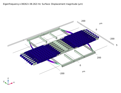
Find the Studies subsection. In the Select Study tree, select Preset Studies for Selected Physics Interfaces>Eigenfrequency, Prestressed.
|
|
4
|
|
5
|
|
1
|
|
2
|
In the Settings window for Study, type Study 2 - Prestressed Eigenfrequency in the Label text field.
|
|
1
|
|
2
|
|
3
|
|
1
|
|
2
|
|
3
|
|
4
|
|
5
|
|
6
|
|
1
|
|
1
|
|
2
|
In the Settings window for Parameters, type Parameters 3 - Estimate drive mode frequency in the Label text field.
|
|
3
|
Locate the Parameters section. In the table, enter the following settings:
|
|
1
|
|
2
|
In the Settings window for Parameters, type Parameters 4 - Estimate sense mode frequency in the Label text field.
|
|
3
|
Locate the Parameters section. In the table, enter the following settings:
|
|
1
|
|
2
|
In the Settings window for Parameters, type Parameters 5 - Result from Study 2 in the Label text field.
|
|
3
|
Locate the Parameters section. In the table, enter the following settings:
|
|
1
|
|
2
|
|
3
|
Find the Studies subsection. In the Select Study tree, select Preset Studies for Selected Physics Interfaces>Frequency Domain, Prestressed.
|
|
4
|
|
5
|
|
1
|
|
2
|
In the Settings window for Study, type Study 3 - Prestressed Frequency Domain in the Label text field.
|
|
1
|
|
2
|
|
3
|
|
1
|
|
2
|
|
3
|
|
4
|
|
5
|
|
6
|
Click
|
|
8
|
Click
|
|
10
|
|
1
|
|
2
|
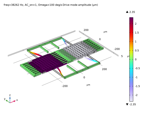
In the Settings window for 3D Plot Group, type Imag X displacement - Drive mode amplitude in the Label text field.
|
|
3
|
|
4
|
|
5
|
|
6
|
|
1
|
In the Model Builder window, expand the Imag X displacement - Drive mode amplitude node, then click Volume 1.
|
|
2
|
|
3
|
|
1
|
|
2
|
|
3
|
|
4
|
|
5
|
|
6
|
|
1
|
|
2
|
In the Settings window for Parameters, type Parameters 6 - Estimate drive mode amplitude in the Label text field.
|
|
3
|
Locate the Parameters section. In the table, enter the following settings:
|
|
1
|
|
2
|
In the Settings window for 3D Plot Group, type Real Z displacement - No rotation in the Label text field.
|
|
3
|
|
4
|
|
5
|
|
1
|
In the Model Builder window, expand the Real Z displacement - No rotation node, then click Volume 1.
|
|
2
|
|
3
|
|
4
|
|
1
|
|
2
|
|
3
|
|
4
|
|
1
|
|
2
|
In the Settings window for 3D Plot Group, type Real Z Displacement - Rotation in the Label text field.
|
|
3
|
|
4
|
|
1
|
|
2
|
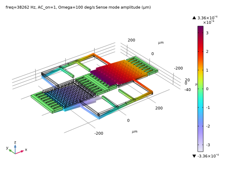
In the Settings window for 3D Plot Group, type Real Z displacement - Net sense signal in the Label text field.
|
|
3
|
|
4
|
|
1
|
In the Model Builder window, expand the Real Z displacement - Net sense signal node, then click Volume 1.
|
|
2
|
|
3
|
|
1
|
|
2
|
|
3
|
|
4
|
|
5
|
|
6
|
|
1
|
|
2
|
In the Settings window for Parameters, type Parameters 7 - Estimate sense mode amplitude in the Label text field.
|
|
3
|
Locate the Parameters section. In the table, enter the following settings:
|
|
1
|
|
2
|
|
3
|
|
4
|
|
5
|
|
1
|
|
2
|
In the Settings window for Evaluation Group, type Evaluation Group 1 - Study 1 - Stationary in the Label text field.
|
|
1
|
|
2
|
|
4
|
|
1
|
In the Model Builder window, right-click Evaluation Group 1 - Study 1 - Stationary and choose Duplicate.
|
|
2
|
In the Settings window for Evaluation Group, type Evaluation Group 2 - Study 3 - Prestressed Frequency Domain in the Label text field.
|
|
3
|
Locate the Data section. From the Dataset list, choose Study 3 - Prestressed Frequency Domain/Solution 4 (sol4).
|
|
4
|
|
1
|
In the Model Builder window, expand the Evaluation Group 2 - Study 3 - Prestressed Frequency Domain node, then click Global Evaluation 1.
|
|
2
|
|
4
|
|
5
|