You are viewing the documentation for an older COMSOL version. The latest version is available here.
PDF

Component Mode Synthesis Tutorial
Introduction
In this tutorial example, the concepts of Component Mode Synthesis (CMS) are introduced through a simple solid model of a cantilever beam. Parts of the beam are reduced by the CMS technique. It is, furthermore, shown how CMS can be used to represent both the static and dynamic behavior of the entire assembly by studying the damped free vibration of the beam. The example, moreover, explores two different ways of applying loads on reduced components.
To verify the validity of the model reduced by CMS, its results are compared to those from a full (unreduced) version of the model.
Model Definition
The model consists of a 3 m long cantilever beam with a rectangular cross section of dimension 0.15-by-0.2 m. In order to show the CMS reduction technique, the beam is split into three 1 m long parts, or components, as seen in Figure 1. When working with CMS, disconnected components are connected using Attachment nodes combined with joints. In this example, they are rigidly connected using a Fixed Joint.
Figure 1: Geometry of the model showing three components and the applied loads.
All three components are considered to be elastic and have viscous damping with material properties according to Table 1. The Young’s modulus of component 2 is, however, made dependent on the axial strain εXX; this nonlinearity means that it cannot be reduced by the CMS technique.
ρ
7850
200
0.3
ηb
50
ηv
20
The analysis includes two study steps:
1
2
To define the boundary conditions, a fixed constraint is applied to the free end of component 1 and two distributed loads are applied to the beam, as can be seen in Figure 1. The load in the y direction is given a magnitude of 0.1 MPa and is kept constant throughout both steps. The load in the z direction is applied to the free end of component 3 and is given a magnitude of 1 MPa, but it is only active during the stationary step. Hence, as the load is removed as the beam starts to vibrate.
Moreover, the analysis is run in two configurations:
1
2
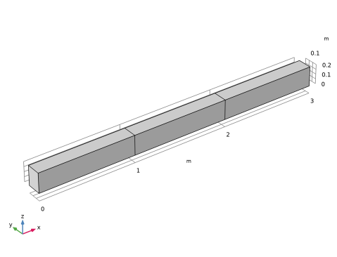
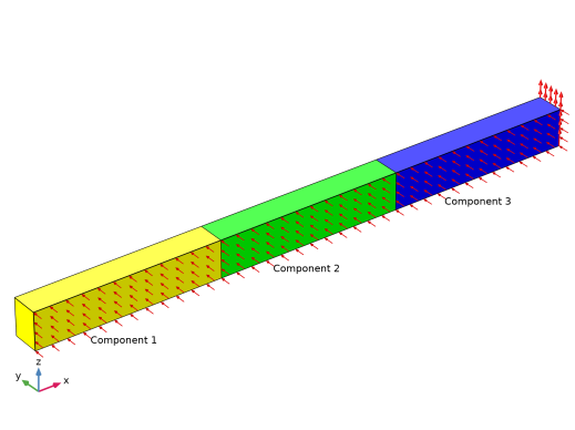
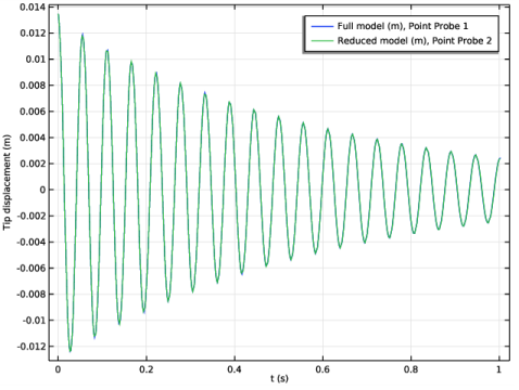
Components 1 and 3 are reduced using CMS, while component 2 is unreduced. This corresponds to a hybrid CMS and FEM solution to the problem.
When working with CMS, the full static and dynamic behavior of a component is represented by a number of constrained eigenmodes, and static constraint modes. These are independent of each other and are used to construct a so-called reduced-order model (ROM) for each reduced component. In essence, the ROM consists of small stiffness and mass matrices, designed so that the static stiffness, inertial properties, and characteristic dynamic properties are maintained. The ROM can also contain other information, such as loads applied on the reduced component.
The number of eigenmodes must be sufficiently large so that the dynamics of the component can be represented accurately. In this example, six eigenmodes are used when reducing components 1 and 3. This is enough to describe the first four bending modes, one twisting mode, and one axial extension mode as shown in Figure 2.
Figure 2: The six constrained eigenmodes.
The number of constraint modes depends on the connections to other parts of the model; in COMSOL Multiphysics, the number of Attachment nodes. In this example, component 1 has one such node to connect it to component 2. For component 3, two Attachment nodes are used, even though there is only one connection to another component. This exemplifies that an Attachment node does not have to be connected to other parts of the model, but can also be used to make it possible for the reduced component to represent additional static modes. Here the extra attachment is needed to represent the static deformation caused by the two loads. A set of six constraint modes is shown in Figure 3. This represents all modes related to one Attachment node.
Figure 3: The six constraint modes for one of the Attachment nodes of component 3.
The constraint modes are generated by setting each attachment degree of freedom to 1 while the others are fixed. Thus, an attachment in 3D will give six constraint modes (three translations and three rotations). In 2D, there will be three constraint modes.
Results and Discussion
Figure 4 shows the tip displacement of the cantilever beam during the time dependent step for both the full solution, and while using the CMS technique. The agreement is in general very good, but a small phase shift can be observed for the reduced model.
It is possible to visualize all result variables also in the reduced components. Hence, we can compare, for example, the von Mises stress in the two configurations. This is shown in Figure 5 and Figure 6, where the stress level in the beam at t = 0 is displayed for the full and reduced model, respectively. The stress level is practically identical for the two configurations. In the figures, the effect of connecting the components by attachments and rigid connections is clearly visible as a disturbance in the stress field at the transition between components 1 and 2 for both configurations.
Figure 4: Tip displacement for both configurations of the analysis.
Figure 5: Distribution of the von Mises stress at t = 0 for the full (unreduced) model.
Figure 6: Distribution of the von Mises stress at t = 0 for the reduced model.
Notes About the COMSOL Implementation
When setting up the reduced model, the two boundary loads actually represent two different ways of applying loads to a reduced component:
1
The contribution of the load in the y direction is applied external to the ROM.
2
The contribution of the load in the z direction is internal to the ROM, and is parameterized by a control variable.
While possible, it is normally not best practice to mix these two methods in the same model. In this example, this is nevertheless done in order to showcase them both. In most cases, the first method is preferable as it provides more flexibility, but in some cases it can be more expensive when performing the global analysis.
For this small example, solving the full model is actually faster than the reduced model. This follows from the extra work related to the ROMs that represent the reduced components. As the model size increases, the extra work related to the ROMs scales better than solving the full model, and one can expect improved performance when using CMS.
Application Library path: MEMS_Module/Dynamics_and_Vibration/cms_tutorial
Modeling Instructions
From the File menu, choose New.
New
In the New window, click  Model Wizard.
Model Wizard
1
In the Model Wizard window, click  3D.
2
In the Select Physics tree, select Structural Mechanics>Solid Mechanics (solid).
3
Click Add.
4
Click  Study.
5
In the Select Study tree, select General Studies>Stationary.
6
Geometry 1
Block 1 (blk1)
1
In the Geometry toolbar, click  Block.
2
In the Settings window for Block, locate the Size and Shape section.
3
In the Depth text field, type 0.15.
4
In the Height text field, type 0.2.
Array 1 (arr1)
1
In the Geometry toolbar, click  Transforms and choose Array.
2
3
In the Settings window for Array, locate the Size section.
4
In the x size text field, type 3.
5
Locate the Displacement section. In the x text field, type 1.
Form Union (fin)
Create an assembly so that selected parts can be reduced.
1
In the Model Builder window, under Component 1 (comp1)>Geometry 1 click Form Union (fin).
2
In the Settings window for Form Union/Assembly, locate the Form Union/Assembly section.
3
From the Action list, choose Form an assembly.
4
Clear the Create pairs check box.
5
In the Geometry toolbar, click  Build All.
Solid Mechanics (solid)
Linear Elastic Material 1
In the Model Builder window, under Component 1 (comp1)>Solid Mechanics (solid) click Linear Elastic Material 1.
Damping 1
1
In the Physics toolbar, click  Attributes and choose Damping.
2
In the Settings window for Damping, locate the Damping Settings section.
3
From the Damping type list, choose Viscous damping.
4
In the ηb text field, type 5e7.
5
In the ηv text field, type 2e7.
Fixed Constraint 1
1
In the Physics toolbar, click  Boundaries and choose Fixed Constraint.
2
Connect the assembly parts with Attachment and Fixed Joint nodes. An Attachment is added to the free end with no constraints; this is only necessary when later building the reduced model in order to capture all deformation modes during model reduction.
Attachment 1
1
In the Physics toolbar, click  Boundaries and choose Attachment.
2
Attachment 2
1
Right-click Attachment 1 and choose Duplicate.
2
Fixed Joint 1
1
In the Physics toolbar, click  Global and choose Fixed Joint.
2
In the Settings window for Fixed Joint, locate the Attachment Selection section.
3
From the Source list, choose Attachment 1.
4
From the Destination list, choose Attachment 2.
Attachment 3
1
In the Physics toolbar, click  Boundaries and choose Attachment.
2
Attachment 4
1
Right-click Attachment 3 and choose Duplicate.
2
Fixed Joint 2
1
In the Physics toolbar, click  Global and choose Fixed Joint.
2
In the Settings window for Fixed Joint, locate the Attachment Selection section.
3
From the Source list, choose Attachment 3.
4
From the Destination list, choose Attachment 4.
Attachment 5
1
In the Physics toolbar, click  Boundaries and choose Attachment.
2
Apply a boundary load at the free end of the cantilever beam. The force per unit area in the z direction will be controlled by a parameter load in the study steps.
Global Definitions
Parameters 1
1
In the Model Builder window, under Global Definitions click Parameters 1.
2
In the Settings window for Parameters, locate the Parameters section.
3
Solid Mechanics (solid)
Boundary Load 1
1
In the Physics toolbar, click  Boundaries and choose Boundary Load.
2
3
In the Settings window for Boundary Load, locate the Force section.
4
Specify the FA vector as
Apply a constant boundary load on one of the sides of the beam.
Boundary Load 2
1
In the Physics toolbar, click  Boundaries and choose Boundary Load.
2
3
In the Settings window for Boundary Load, locate the Force section.
4
Specify the FA vector as
Materials
Material, Linear
1
In the Model Builder window, under Component 1 (comp1) right-click Materials and choose Blank Material.
2
In the Settings window for Material, type Material, Linear in the Label text field.
3
Locate the Material Contents section. In the table, enter the following settings:
Make the material of the middle part nonlinear by defining Young’s modulus as a function of the axial strain.
Material, Linear 1 (mat2)
1
Right-click Material, Linear and choose Duplicate.
2
Definitions
Step 1 (step1)
1
In the Home toolbar, click  Functions and choose Local>Step.
2
In the Settings window for Step, locate the Parameters section.
3
In the From text field, type 0.8.
4
In the To text field, type 1.2.
5
Click to expand the Smoothing section. In the Size of transition zone text field, type 1e-3.
Materials
Material, Nonlinear
1
In the Model Builder window, under Component 1 (comp1)>Materials click Material, Linear 1 (mat2).
2
In the Settings window for Material, type Material, Nonlinear in the Label text field.
3
Locate the Material Contents section. In the table, enter the following settings:
Create a structured mesh.
Mesh 1
Mapped 1
1
In the Mesh toolbar, click  Boundary and choose Mapped.
2
Distribution 1
1
Right-click Mapped 1 and choose Distribution.
2
In the Settings window for Distribution, locate the Edge Selection section.
3
From the Selection list, choose All edges.
4
Locate the Distribution section. In the Number of elements text field, type 4.
Swept 1
In the Mesh toolbar, click  Swept.
Distribution 1
1
Right-click Swept 1 and choose Distribution.
2
In the Settings window for Distribution, locate the Distribution section.
3
In the Number of elements text field, type 12.
4
Click  Build All.
The first study will be used to compute the full (unreduced) model of the beam. Add a Time Dependent study step to Study 1. Use the parameter load to apply a vertical load of 1 MPa at the free end during the stationary step. The load is then removed to study the damped free vibration of the beam.
Study, Full Model
1
In the Model Builder window, click Study 1.
2
In the Settings window for Study, type Study, Full Model in the Label text field.
Time Dependent
1
In the Study toolbar, click  Study Steps and choose Time Dependent>Time Dependent.
2
In the Settings window for Time Dependent, locate the Study Settings section.
3
In the Output times text field, type range(0,0.05,1).
Step 1: Stationary
1
In the Model Builder window, click Step 1: Stationary.
2
In the Settings window for Stationary, click to expand the Study Extensions section.
3
Select the Auxiliary sweep check box.
4
5
6
From the Run continuation for list, choose No parameter.
Step 2: Time Dependent
1
In the Model Builder window, click Step 2: Time Dependent.
2
In the Settings window for Time Dependent, click to expand the Study Extensions section.
3
Select the Auxiliary sweep check box.
4
5
Create a Point Probe to monitor the vertical displacement of the free end.
Definitions
Point Probe 1 (point1)
1
In the Definitions toolbar, click  Probes and choose Point Probe.
2
In the Settings window for Point Probe, locate the Source Selection section.
3
Click  Clear Selection.
4
5
Locate the Expression section. In the Expression text field, type w.
6
Select the Description check box. In the associated text field, type Full model.
Study, Full Model
Step 1: Stationary
1
In the Model Builder window, under Study, Full Model click Step 1: Stationary.
2
In the Settings window for Stationary, click to expand the Results While Solving section.
3
From the Probes list, choose None.
4
In the Home toolbar, click  Compute.
You will now use Component Mode Synthesis and model reduction to reduce the number of degrees of freedom of the two linear parts of the assembly. Any number of linear parts of the assembly can be reduced using a Reduced Flexible Components node. In this example, the middle part of the beam is nonlinear and cannot be reduced. Disconnected parts of the selection are automatically detected and identified as individual components.
Solid Mechanics (solid)
Reduced Flexible Components 1
1
In the Physics toolbar, click  Domains and choose Reduced Flexible Components.
2
The load at the free end will in this tutorial be part of the ROM. To control its amplitude, add a control variable load in a Global Reduced Model Input node; enable Reduced-Order Modeling in the Show More Options dialog to show it. Using the name of an existing model parameter will redefine that parameter as a reduced model input with value linked from the parameter’s original definition.
3
Click the  Show More Options button in the Model Builder toolbar.
4
In the Show More Options dialog box, select Study>Reduced-Order Modeling in the tree.
5
6
Global Definitions
Global Reduced-Model Inputs 1
1
In the Physics toolbar, click  Reduced-Order Modeling and choose Global Reduced-Model Inputs.
2
In the Settings window for Global Reduced-Model Inputs, locate the Reduced-Model Inputs section.
3
Solid Mechanics (solid)
Reduced Flexible Components 1
You can automatically set up a study sequence for the model reduction of each component from the Reduced Flexible Components node. Use six eigenmodes for both components.
1
In the Model Builder window, under Component 1 (comp1)>Solid Mechanics (solid) click Reduced Flexible Components 1.
2
In the Settings window for Reduced Flexible Components, locate the Component Mode Synthesis section.
3
In the Number of eigenmodes text field, type 6.
4
Click CMS Configuration in the upper-right corner of the Component Mode Synthesis section. From the menu, choose Configure CMS Study.
Boundary Load 1 should be part of the reduced component and needs to be enabled in the reference study step of the Model Reduction step.
CMS Study
In the Model Builder window, expand the CMS Study node.
Time Dependent
1
In the Model Builder window, expand the CMS Study>Step 3: Model Reduction node, then click Time Dependent.
2
In the Settings window for Time Dependent, locate the Physics and Variables Selection section.
3
In the tree, select Component 1 (comp1)>Solid Mechanics (solid)>Boundary Load 1.
4
Compute the CMS Study to generate the reduced components.
5
In the Home toolbar, click  Compute.
Now, create a study for performing the same analysis as in Study, Full Model, but with reduced components.
Add Study
1
In the Home toolbar, click  Add Study to open the Add Study window.
2
Go to the Add Study window.
3
Find the Studies subsection. In the Select Study tree, select Empty Study.
4
Click Add Study in the window toolbar.
5
In the Home toolbar, click  Add Study to close the Add Study window.
Study, Reduced Model
In the Settings window for Study, type Study, Reduced Model in the Label text field.
Study, Full Model
Step 1: Stationary, Step 2: Time Dependent
1
In the Model Builder window, under Study, Full Model, Ctrl-click to select Step 1: Stationary and Step 2: Time Dependent.
2
Study, Reduced Model
Step 1: Stationary
1
In the Model Builder window, right-click Study, Reduced Model and choose Paste Multiple Items.
Boundary Load 1 should not be active in Study, Reduced Model, since it is already part of Reduced Component 2. Note that Boundary Load 2 adds a load on both reduced and unreduced parts of the assembly.
2
In the Settings window for Stationary, locate the Physics and Variables Selection section.
3
Select the Modify model configuration for study step check box.
4
In the tree, select Component 1 (comp1)>Solid Mechanics (solid)>Boundary Load 1.
5
Step 2: Time Dependent
1
In the Model Builder window, click Step 2: Time Dependent.
2
In the Settings window for Time Dependent, locate the Physics and Variables Selection section.
3
Select the Modify model configuration for study step check box.
4
In the tree, select Component 1 (comp1)>Solid Mechanics (solid)>Boundary Load 1.
5
Duplicate Point Probe 1 to also monitor the vertical displacement when solving the reduced model.
Definitions
Point Probe 2 (point2)
1
In the Model Builder window, under Component 1 (comp1)>Definitions right-click Point Probe 1 (point1) and choose Duplicate.
2
In the Settings window for Point Probe, locate the Expression section.
3
In the Description text field, type Reduced model.
4
Click to expand the Table and Window Settings section. From the Output table list, choose New table.
Study, Reduced Model
Step 2: Time Dependent
1
In the Model Builder window, under Study, Reduced Model click Step 2: Time Dependent.
2
In the Settings window for Time Dependent, click to expand the Results While Solving section.
3
From the Probes list, choose Manual.
4
In the Probes list, select Point Probe 1 (point1).
5
Under Probes, click  Delete.
6
In the Home toolbar, click  Compute.
Create plots to visualize the constrained eigenmodes and some of the constraint modes for Reduced Component 2. The solution datasets of the CMS study contains the results from the last component in the sweep, where CMS Study/Solution Store 1 contains the constraint modes and CMS Study/Solution Store 2 the eigenmodes.
Results
Constrained Eigenmodes
1
In the Home toolbar, click  Add Plot Group and choose 3D Plot Group.
2
In the Settings window for 3D Plot Group, type Constrained Eigenmodes in the Label text field.
3
Locate the Data section. From the Dataset list, choose CMS Study/Solution Store 3 (sol5).
4
Click to expand the Title section. From the Title type list, choose None.
5
Locate the Color Legend section. Clear the Show legends check box.
6
Click to expand the Plot Array section. Select the Enable check box.
7
From the Array shape list, choose Square.
8
From the Order list, choose Column-major.
Volume 1
1
Right-click Constrained Eigenmodes and choose Volume.
2
In the Settings window for Volume, locate the Coloring and Style section.
3
Click  Change Color Table.
4
In the Color Table dialog box, select Wave>DiscoLight in the tree.
5
Deformation 1
Right-click Volume 1 and choose Deformation.
Volume 2
1
In the Model Builder window, under Results>Constrained Eigenmodes right-click Volume 1 and choose Duplicate.
2
In the Settings window for Volume, locate the Data section.
3
From the Dataset list, choose CMS Study/Solution Store 3 (sol5).
4
From the Eigenfrequency (Hz) list, choose 852.06.
Volume 3
1
Right-click Volume 2 and choose Duplicate.
2
In the Settings window for Volume, locate the Data section.
3
From the Eigenfrequency (Hz) list, choose 1407.1.
Volume 4
1
Right-click Volume 3 and choose Duplicate.
2
In the Settings window for Volume, locate the Data section.
3
From the Eigenfrequency (Hz) list, choose 1680.2.
Volume 5
1
Right-click Volume 4 and choose Duplicate.
2
In the Settings window for Volume, locate the Data section.
3
From the Eigenfrequency (Hz) list, choose 1952.3.
Volume 6
1
Right-click Volume 5 and choose Duplicate.
2
In the Settings window for Volume, locate the Data section.
3
From the Eigenfrequency (Hz) list, choose 2550.5.
4
In the Constrained Eigenmodes toolbar, click  Plot.
5
Click the  Zoom Extents button in the Graphics toolbar.
6
Click the  Show Grid button in the Graphics toolbar.
Constraint Modes
1
In the Home toolbar, click  Add Plot Group and choose 3D Plot Group.
2
In the Settings window for 3D Plot Group, type Constraint Modes in the Label text field.
3
Locate the Data section. From the Dataset list, choose CMS Study/Solution Store 2 (sol4).
4
Locate the Title section. From the Title type list, choose None.
5
Locate the Color Legend section. Clear the Show legends check box.
6
Locate the Plot Array section. Select the Enable check box.
7
From the Array shape list, choose Square.
8
From the Order list, choose Column-major.
Volume 1
1
Right-click Constraint Modes and choose Volume.
2
In the Settings window for Volume, locate the Data section.
3
From the Dataset list, choose CMS Study/Solution Store 2 (sol4).
4
From the Parameter value (c_rfc1_solid) list, choose 1.
5
Locate the Coloring and Style section. Click  Change Color Table.
6
In the Color Table dialog box, select Rainbow>SpectrumLight in the tree.
7
Deformation 1
Right-click Volume 1 and choose Deformation.
Volume 2
1
In the Model Builder window, under Results>Constraint Modes right-click Volume 1 and choose Duplicate.
2
In the Settings window for Volume, locate the Data section.
3
From the Parameter value (c_rfc1_solid) list, choose 2.
Volume 3
1
Right-click Volume 2 and choose Duplicate.
2
In the Settings window for Volume, locate the Data section.
3
From the Parameter value (c_rfc1_solid) list, choose 3.
Volume 4
1
Right-click Volume 3 and choose Duplicate.
2
In the Settings window for Volume, locate the Data section.
3
From the Parameter value (c_rfc1_solid) list, choose 4.
Volume 5
1
Right-click Volume 4 and choose Duplicate.
2
In the Settings window for Volume, locate the Data section.
3
From the Parameter value (c_rfc1_solid) list, choose 5.
Volume 6
1
Right-click Volume 5 and choose Duplicate.
2
In the Settings window for Volume, locate the Data section.
3
From the Parameter value (c_rfc1_solid) list, choose 6.
4
In the Constraint Modes toolbar, click  Plot.
5
Click the  Zoom Extents button in the Graphics toolbar.
Modify the default stress plots to show the stress level when all loads are applied.
Stress (solid)
1
In the Model Builder window, under Results click Stress (solid).
2
In the Settings window for 3D Plot Group, locate the Data section.
3
From the Time (s) list, choose 0.
4
In the Stress (solid) toolbar, click  Plot.
5
Click the  Zoom Extents button in the Graphics toolbar.
Stress (solid) 1
1
In the Model Builder window, click Stress (solid) 1.
2
In the Settings window for 3D Plot Group, locate the Data section.
3
From the Time (s) list, choose 0.
4
In the Stress (solid) 1 toolbar, click  Plot.
5
Click the  Zoom Extents button in the Graphics toolbar.
To be able to recompute Study, Full Model with the same setting as before, disable Reduced Flexible Components and the ROMs that were added for Study, Reduced Model.
Study, Full Model
Step 1: Stationary
1
In the Model Builder window, under Study, Full Model click Step 1: Stationary.
2
In the Settings window for Stationary, locate the Physics and Variables Selection section.
3
Select the Modify model configuration for study step check box.
4
In the tree, select Global Definitions>Reduced-Order Modeling>Reduced Component 1 (rom1_n_rfc1_solid_1) and Global Definitions>Reduced-Order Modeling>Reduced Component 2 (rom1_n_rfc1_solid_2).
5
Right-click and choose Disable in Model.
6
In the tree, select Component 1 (comp1)>Solid Mechanics (solid)>Reduced Flexible Components 1.
7
Step 2: Time Dependent
1
In the Model Builder window, click Step 2: Time Dependent.
2
In the Settings window for Time Dependent, click to expand the Results While Solving section.
3
From the Probes list, choose Manual.
4
In the Probes list, select Point Probe 2 (point2).
5
Under Probes, click  Delete.
6
Locate the Physics and Variables Selection section. Select the Modify model configuration for study step check box.
7
In the tree, select Global Definitions>Reduced-Order Modeling>Reduced Component 1 (rom1_n_rfc1_solid_1) and Global Definitions>Reduced-Order Modeling>Reduced Component 2 (rom1_n_rfc1_solid_2).
8
Right-click and choose Disable in Model.
9
In the tree, select Component 1 (comp1)>Solid Mechanics (solid)>Reduced Flexible Components 1.
10