|
|
|
|
•
|


|
•
|
Use the Mass and Moment of Inertia subnode of the Rigid Material node to enter the inertia properties given at a certain point.
|
|
•
|
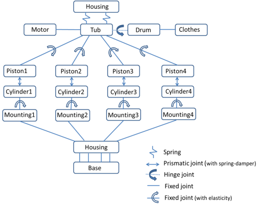
The connections set up in the model and the details of the system DOF and constraints can be seen in the Joints Summary and Rigid Body DOF Summary sections of the Multibody Dynamics node.
|
|
•
|
Use the Attachment boundary condition in the Shell interface to establish the connection to the solid objects through joints and springs.
|
|
1
|
|
2
|
|
3
|
Click Add.
|
|
4
|
|
5
|
Click Add.
|
|
6
|
Click
|
|
7
|
|
8
|
Click
|
|
1
|
|
2
|
|
3
|
|
4
|
Browse to the model’s Application Libraries folder and double-click the file washing_machine_vibration_parameters.txt.
|
|
1
|
|
2
|
|
3
|
|
1
|
|
2
|
|
3
|
Click
|
|
4
|
Browse to the model’s Application Libraries folder and double-click the file washing_machine_vibration.mphbin.
|
|
5
|
Click
|
|
1
|
|
2
|
|
3
|
|
4
|
|
5
|
|
1
|
|
2
|
|
3
|
|
1
|
|
2
|
|
3
|
|
4
|
|
1
|
|
2
|
|
3
|
|
5
|
|
1
|
|
2
|
|
3
|
|
5
|
|
1
|
|
2
|
|
3
|
|
1
|
|
2
|
|
3
|
|
1
|
|
2
|
|
3
|
|
1
|
In the Model Builder window, under Component 1 (comp1) right-click Multibody Dynamics (mbd) and choose Material Models>Rigid Material.
|
|
2
|
|
4
|
|
1
|
|
2
|
In the Settings window for Mass and Moment of Inertia, locate the Mass and Moment of Inertia section.
|
|
3
|
|
1
|
|
2
|
|
3
|
Specify the F vector as
|
|
1
|
|
2
|
|
4
|
|
5
|
|
6
|
|
7
|
|
8
|
|
9
|
|
1
|
|
2
|
|
3
|
|
4
|
|
5
|
|
1
|
|
1
|
|
2
|
|
1
|
|
2
|
|
4
|
|
1
|
|
2
|
In the Settings window for Mass and Moment of Inertia, locate the Mass and Moment of Inertia section.
|
|
3
|
|
4
|
|
1
|
|
2
|
|
1
|
In the Model Builder window, under Component 1 (comp1) right-click Materials and choose Blank Material.
|
|
2
|
|
1
|
|
2
|
|
3
|
In the tree, select Built-in>Aluminum.
|
|
4
|
|
5
|
|
1
|
|
2
|
|
3
|
|
1
|
|
2
|
|
3
|
|
4
|
|
1
|
In the Model Builder window, under Component 1 (comp1)>Shell [Housing] (shell) click Thickness and Offset 1.
|
|
2
|
|
3
|
|
1
|
|
2
|
|
3
|
|
1
|
|
2
|
|
1
|
|
2
|
|
3
|
|
4
|
|
1
|
|
1
|
|
2
|
|
3
|
|
1
|
In the Model Builder window, expand the Component 1 (comp1)>Multibody Dynamics (mbd)>Housing-tub (back) node, then click Destination Point 1.
|
|
2
|
|
3
|
|
1
|
|
2
|
|
3
|
|
4
|
|
5
|
|
6
|
|
1
|
|
1
|
|
2
|
|
3
|
|
4
|
|
1
|
|
2
|
|
3
|
|
4
|
|
1
|
|
1
|
|
2
|
|
3
|
|
4
|
|
1
|
|
2
|
|
3
|
|
1
|
|
2
|
|
3
|
|
4
|
|
5
|
|
1
|
|
1
|
|
2
|
|
3
|
|
1
|
|
2
|
|
3
|
|
4
|
|
1
|
|
2
|
|
3
|
|
4
|
|
5
|
|
6
|
|
1
|
|
1
|
|
2
|
|
3
|
|
1
|
|
2
|
|
3
|
|
4
|
|
5
|
|
6
|
|
7
|
|
1
|
In the Model Builder window, under Component 1 (comp1)>Multibody Dynamics (mbd) click Cylinder 2-piston 2.
|
|
2
|
|
3
|
|
1
|
|
2
|
|
3
|
|
1
|
|
2
|
|
3
|
|
1
|
|
2
|
|
3
|
|
1
|
|
2
|
|
3
|
|
1
|
|
2
|
|
3
|
|
1
|
|
2
|
|
3
|
|
4
|
|
5
|
|
6
|
|
7
|
|
1
|
|
2
|
|
3
|
|
4
|
|
1
|
|
2
|
|
3
|
|
4
|
|
5
|
|
6
|
|
7
|
|
1
|
|
2
|
|
1
|
|
2
|
|
3
|
|
4
|
|
5
|
Click OK.
|
|
1
|
|
2
|
|
3
|
|
4
|
|
5
|
|
6
|
|
7
|
Click OK.
|
|
8
|
|
9
|
|
1
|
|
2
|
|
3
|
|
4
|
|
5
|
|
1
|
|
2
|
|
3
|
|
4
|
|
5
|
|
6
|
|
7
|
|
8
|
|
1
|
In the Model Builder window, under Component 1 (comp1) right-click Definitions and choose Variables.
|
|
2
|
|
1
|
|
2
|
|
3
|
|
4
|
|
5
|
|
1
|
|
2
|
|
3
|
|
4
|
|
5
|
|
1
|
|
2
|
|
3
|
|
4
|
|
5
|
Click to expand the Time Stepping section. From the Steps taken by solver list, choose Intermediate.
|
|
6
|
Right-click Study 2>Solver Configurations>Solution 2 (sol2)>Time-Dependent Solver 1 and choose Fully Coupled.
|
|
7
|
|
8
|
|
9
|
|
10
|
In the Model Builder window, under Study 2>Solver Configurations>Solution 2 (sol2)>Time-Dependent Solver 1 click Advanced.
|
|
11
|
|
12
|
|
13
|
|
1
|
|
2
|
|
3
|
|
4
|
|
5
|
|
6
|
|
1
|
In the Model Builder window, expand the Results>Displacement>Surface 1 node, then click Deformation 1.
|
|
2
|
|
3
|
|
1
|
In the Model Builder window, expand the Results>Displacement>Surface 2 node, then click Deformation 1.
|
|
2
|
|
3
|
|
4
|
|
5
|
|
1
|
|
2
|
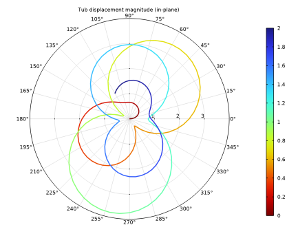
In the Settings window for Polar Plot Group, type Tub displacement magnitude (in-plane) in the Label text field.
|
|
3
|
|
4
|
|
1
|
|
2
|
In the Settings window for Global, click Replace Expression in the upper-right corner of the r-Axis Data section. From the menu, choose Component 1 (comp1)>Definitions>Variables>uin_tub - Tub displacement magnitude (in-plane) - m.
|
|
3
|
|
4
|
Click Replace Expression in the upper-right corner of the θ Angle Data section. From the menu, choose Component 1 (comp1)>Definitions>Variables>th_drum - Drum rotation - rad.
|
|
5
|
|
6
|
|
1
|
|
2
|
In the Settings window for Color Expression, click Replace Expression in the upper-right corner of the Expression section. From the menu, choose Solver>t - Time - s.
|
|
3
|
|
4
|
|
5
|
|
1
|
In the Model Builder window, right-click Tub displacement magnitude (in-plane) and choose Duplicate.
|
|
2
|
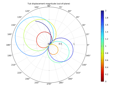
In the Settings window for Polar Plot Group, type Tub displacement magnitude (out-of-plane) in the Label text field.
|
|
1
|
In the Model Builder window, expand the Tub displacement magnitude (out-of-plane) node, then click Global 1.
|
|
2
|
In the Settings window for Global, click Replace Expression in the upper-right corner of the r-Axis Data section. From the menu, choose Component 1 (comp1)>Definitions>Variables>uout_tub - Tub displacement magnitude (out-of-plane) - m.
|
|
3
|
|
4
|
|
1
|
|
2
|
|
3
|
|
4
|
|
5
|
|
6
|
|
7
|
|
1
|
|
2
|
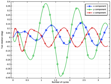
In the Settings window for Global, click Replace Expression in the upper-right corner of the y-Axis Data section. From the menu, choose Component 1 (comp1)>Multibody Dynamics>Rigid domains>Tub>Rigid body rotation (spatial frame) - rad>mbd.rd3.thx - Rigid body rotation, x component.
|
|
3
|
Click Add Expression in the upper-right corner of the y-Axis Data section. From the menu, choose Component 1 (comp1)>Multibody Dynamics>Rigid domains>Tub>Rigid body rotation (spatial frame) - rad>mbd.rd3.thy - Rigid body rotation, y component.
|
|
4
|
Click Add Expression in the upper-right corner of the y-Axis Data section. From the menu, choose Component 1 (comp1)>Multibody Dynamics>Rigid domains>Tub>Rigid body rotation (spatial frame) - rad>mbd.rd3.thz - Rigid body rotation, z component.
|
|
5
|
|
6
|
Click Replace Expression in the upper-right corner of the x-Axis Data section. From the menu, choose Component 1 (comp1)>Definitions>Variables>n_cycle - Number of cycles.
|
|
7
|
|
8
|
|
9
|
|
10
|
|
11
|
|
13
|
|
14
|
|
1
|
|
2
|
In the Settings window for 1D Plot Group, type Stabilizing spring extension in the Label text field.
|
|
3
|
|
4
|
|
1
|
|
2
|
In the Settings window for Global, click Replace Expression in the upper-right corner of the y-Axis Data section. From the menu, choose Component 1 (comp1)>Multibody Dynamics>Spring-Dampers>Housing-tub (front)>mbd.spd1.dl - Spring extension - m.
|
|
3
|
Click Add Expression in the upper-right corner of the y-Axis Data section. From the menu, choose Component 1 (comp1)>Multibody Dynamics>Spring-Dampers>Housing-tub (back) >mbd.spd2.dl - Spring extension - m.
|
|
4
|
Locate the Legends section. In the table, enter the following settings:
|
|
5
|
|
6
|
|
1
|
|
2
|
|
3
|
|
1
|
|
2
|
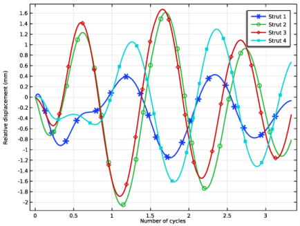
In the Settings window for Global, click Replace Expression in the upper-right corner of the y-Axis Data section. From the menu, choose Component 1 (comp1)>Multibody Dynamics>Prismatic joints>Cylinder 1-piston 1>mbd.prj1.u - Relative displacement - m.
|
|
3
|
Click Add Expression in the upper-right corner of the y-Axis Data section. From the menu, choose Component 1 (comp1)>Multibody Dynamics>Prismatic joints>Cylinder 2-piston 2>mbd.prj2.u - Relative displacement - m.
|
|
4
|
Click Add Expression in the upper-right corner of the y-Axis Data section. From the menu, choose Component 1 (comp1)>Multibody Dynamics>Prismatic joints>Cylinder 3-piston 3>mbd.prj3.u - Relative displacement - m.
|
|
5
|
Click Add Expression in the upper-right corner of the y-Axis Data section. From the menu, choose Component 1 (comp1)>Multibody Dynamics>Prismatic joints>Cylinder 4-piston 4>mbd.prj4.u - Relative displacement - m.
|
|
6
|
Locate the Legends section. In the table, enter the following settings:
|
|
7
|
|
8
|
|
1
|
|
2
|
|
1
|
|
2
|
|
4
|
|
5
|
|
1
|
|
2
|
In the Settings window for 1D Plot Group, type Shell deformation (mountings) in the Label text field.
|
|
3
|
|
1
|
|
2
|
|
4
|
Locate the Legends section. In the table, enter the following settings:
|
|
5
|
|
6
|
|
1
|
|
2
|
|
3
|
|
4
|
|
5
|
|
6
|
|
7
|
|
8
|
Click
|
|
1
|
|
2
|
In the Settings window for 1D Plot Group, type Shell deformation (side wall) in the Label text field.
|
|
3
|
|
4
|
|
5
|
|
6
|
|
7
|
|
8
|
|
1
|
|
2
|
|
3
|
|
4
|
Click Replace Expression in the upper-right corner of the x-Axis Data section. From the menu, choose Component 1 (comp1)>Definitions>Variables>n_cycle - Number of cycles.
|
|
5
|
|
6
|
|
7
|
|
8
|
|
9
|
|
10
|
|
1
|
|
2
|
|
3
|
|
4
|
Locate the Legends section. In the table, enter the following settings:
|
|
1
|
|
2
|
|
3
|
|
4
|
Locate the Legends section. In the table, enter the following settings:
|
|
5
|
|
6
|