PDF

Slider Crank Mechanism
Introduction
In this model you simulate the dynamic behavior of a slider crank mechanism, when the initial velocity of the slider is prescribed and the system is subjected to a gravity load. This is a benchmark problem to test the numerical algorithms in the area of multibody dynamics. This mechanism has only one degree of freedom, but it goes through singular positions during the operation. At the singular position, the mechanism has two instantaneous degrees of freedom, which in general is difficult to handle. The details about the complexity of the problem can be found in Ref. 1.
This model is simulated using the Multibody Dynamics interface and the results of the analysis are compared with those obtained in Ref. 1.
Model Definition
The geometry, which is a simplified version of a slider crank mechanism, is shown in Figure 1. It consists of only two links and the slider is not modeled physically.
Figure 1: Model geometry.
The two links are connected by a hinge joint at point A. One of the links is connected to the ground at point O using a hinge joint. The other one is connected to the ground at point B using a reduced slot joint.
Both links are m long and have a uniformly distributed mass of 1 kg. Initially the crank forms an angle of 45° with the horizontal axis. The slider (point B) is given an initial velocity of 4 m/s in the negative x direction. The whole assembly is subjected to a gravity load, which acts in the negative y direction.
Results and Discussion
The computed results are compared with the solution obtained in Ref. 1. The comparison shows that the computed results are in very good agreement with the results given in the reference.
Figure 2 shows the displacement of the links at t = 10 s and the trajectory of the various points on the arm.
Figure 2: Displacement of the mechanism at t=10 s.
Figure 3: Comparison of the x-component of the acceleration at point A with Ref. 1.
Figure 4: Time variation of kinetic, potential and total energy.
Figure 3 displays the time variation of the acceleration of point A. The computed acceleration is in very good agreement with the values obtained in Ref. 1.
Figure 4 shows the variation of kinetic, potential, and total energy with time. It can be seen that the potential energy is converted into the kinetic energy during the motion and vice-versa, conserving the total energy of the system.
Notes About the COMSOL Implementation
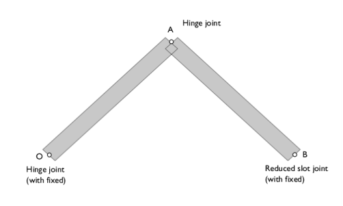
In this model, linkages are modeled as rigid elements using the Rigid Material node as we are only interested in the kinematics of the mechanism.
A Joint node can establish a connection between a Rigid Material or an Attachment node and the ground (Fixed). This helps in avoiding extra geometry components.
The given initial velocity of the slider is enforced by choosing the Force initial values option in the Consistent initialization list found in the Rigid Material node.
Reference
1. E. Bayo and A. Avello, “Singularity-Free Augmented Lagrangian Algorithms for Constrained Multibody Dynamics,” Nonlinear Dynamics, vol. 5, pp. 209–231, 1994.
Application Library path: Multibody_Dynamics_Module/Verification_Examples/slider_crank_mechanism
Modeling Instructions
From the File menu, choose New.
New
In the New window, click  Model Wizard.
Model Wizard
1
In the Model Wizard window, click  2D.
2
In the Select Physics tree, select Structural Mechanics>Multibody Dynamics (mbd).
3
Click Add.
4
Click  Study.
5
In the Select Study tree, select General Studies>Time Dependent.
6
Global Definitions
Parameters 1
1
In the Model Builder window, under Global Definitions click Parameters 1.
2
In the Settings window for Parameters, locate the Parameters section.
3
Geometry 1
Rectangle 1 (r1)
1
In the Geometry toolbar, click  Rectangle.
2
In the Settings window for Rectangle, locate the Size and Shape section.
3
In the Width text field, type d.
4
Locate the Position section. In the x text field, type -d/2.
Rotate 1 (rot1)
1
In the Geometry toolbar, click  Transforms and choose Rotate.
2
3
In the Settings window for Rotate, locate the Rotation section.
4
In the Angle text field, type -45.
Mirror 1 (mir1)
1
In the Geometry toolbar, click  Transforms and choose Mirror.
2
3
In the Settings window for Mirror, locate the Input section.
4
Select the Keep input objects check box.
5
Locate the Point on Line of Reflection section. In the x text field, type l/sqrt(2).
Form Union (fin)
1
In the Model Builder window, under Component 1 (comp1)>Geometry 1 click Form Union (fin).
2
In the Settings window for Form Union/Assembly, locate the Form Union/Assembly section.
3
From the Action list, choose Form an assembly.
4
In the Geometry toolbar, click  Build All.
5
Click the  Zoom Extents button in the Graphics toolbar.
Materials
Material 1 (mat1)
1
In the Model Builder window, under Component 1 (comp1) right-click Materials and choose Blank Material.
Define the density of the material using the mass and geometric-property parameters.
2
In the Settings window for Material, locate the Material Contents section.
3
Multibody Dynamics (mbd)
1
In the Model Builder window, under Component 1 (comp1) click Multibody Dynamics (mbd).
2
In the Settings window for Multibody Dynamics, locate the Thickness section.
3
In the d text field, type d.
Rigid Material 1
1
In the Physics toolbar, click  Domains and choose Rigid Material.
2
Rigid Material 2
1
In the Physics toolbar, click  Domains and choose Rigid Material.
2
Define the initial velocity of the slider and force the same to consistently initialize the remaining degrees of freedom.
3
In the Settings window for Rigid Material, locate the Initial Values section.
4
From the list, choose Locally defined.
5
From the Consistent initialization list, choose Force initial values.
6
Select the Translation along first axis check box.
Initial Values 1
1
In the Model Builder window, expand the Rigid Material 2 node, then click Initial Values.
2
In the Settings window for Initial Values, locate the Initial Values: Translational section.
3
Specify the du/dt vector as
4
5
Locate the Center of Rotation section. From the list, choose Centroid of selected entities.
Center of Rotation: Boundary 1
1
In the Model Builder window, under Component 1 (comp1)>Multibody Dynamics (mbd)>Rigid Material 2>Initial Values 1 click Center of Rotation: Boundary 1.
2
Hinge Joint 1
1
In the Physics toolbar, click  Global and choose Hinge Joint.
2
In the Settings window for Hinge Joint, locate the Attachment Selection section.
3
From the Source list, choose Fixed.
4
From the Destination list, choose Rigid Material 1.
Center of Joint: Boundary 1
1
In the Model Builder window, click Center of Joint: Boundary 1.
2
Hinge Joint 2
1
In the Physics toolbar, click  Global and choose Hinge Joint.
2
In the Settings window for Hinge Joint, locate the Attachment Selection section.
3
From the Source list, choose Rigid Material 1.
4
From the Destination list, choose Rigid Material 2.
Center of Joint: Boundary 1
1
In the Model Builder window, click Center of Joint: Boundary 1.
2
Reduced Slot Joint 1
1
In the Physics toolbar, click  Global and choose Reduced Slot Joint.
2
In the Settings window for Reduced Slot Joint, locate the Attachment Selection section.
3
From the Source list, choose Fixed.
4
From the Destination list, choose Rigid Material 2.
5
Locate the Axes of Joint section. From the Joint translational axis list, choose Attached on source.
The default value of the joint axis can be used here.
Center of Joint: Boundary 1
1
In the Model Builder window, click Center of Joint: Boundary 1.
2
Use the Gravity node to apply the gravity load.
Gravity 1
In the Physics toolbar, click  Global and choose Gravity.
Mesh 1
Since both components are rigid, a single element is sufficient for computing the inertial properties.
Mapped 1
In the Mesh toolbar, click  Mapped.
Distribution 1
1
Right-click Mapped 1 and choose Distribution.
2
In the Settings window for Distribution, locate the Boundary Selection section.
3
From the Selection list, choose All boundaries.
4
Locate the Distribution section. In the Number of elements text field, type 1.
5
Click  Build All.
Definitions
Integration 1 (intop1)
1
In the Definitions toolbar, click  Nonlocal Couplings and choose Integration.
2
Click in the Graphics window and then press Ctrl+A to select both domains.
Variables 1
1
In the Definitions toolbar, click  Local Variables.
2
In the Settings window for Variables, locate the Variables section.
3
Study 1
Step 1: Time Dependent
1
In the Model Builder window, under Study 1 click Step 1: Time Dependent.
2
In the Settings window for Time Dependent, locate the Study Settings section.
3
In the Output times text field, type range(0,0.005,10).
Increase the BDF order for the accurate evaluation of acceleration.
Solution 1 (sol1)
1
In the Study toolbar, click  Show Default Solver.
2
In the Model Builder window, expand the Solution 1 (sol1) node, then click Time-Dependent Solver 1.
3
In the Settings window for Time-Dependent Solver, click to expand the Time Stepping section.
4
From the Maximum BDF order list, choose 3.
5
In the Study toolbar, click  Compute.
The two default plots show the displacement and velocity profile of the slider crank mechanism. Add the trajectories of the points on the arm to the first default plot shown in Figure 2.
Create the cut points on the arm at various locations to plot the trajectory.
Results
Cut Point 2D 1
1
In the Results toolbar, click  Cut Point 2D.
2
In the Settings window for Cut Point 2D, locate the Point Data section.
3
In the X text field, type 1/sqrt(2) 1.5/sqrt(2) sqrt(2).
4
In the Y text field, type 1/sqrt(2) 0.5/sqrt(2) 0.
Cut Point 2D 2
1
Right-click Cut Point 2D 1 and choose Duplicate.
2
In the Settings window for Cut Point 2D, locate the Point Data section.
3
In the X text field, type 1/sqrt(2).
4
In the Y text field, type 1/sqrt(2).
Displacement (mbd)
In the Model Builder window, under Results click Displacement (mbd).
Point Trajectories 1
1
In the Displacement (mbd) toolbar, click  More Plots and choose Point Trajectories.
2
In the Settings window for Point Trajectories, locate the Data section.
3
From the Dataset list, choose Cut Point 2D 1.
4
From the Solution parameters list, choose From parent.
5
Locate the Coloring and Style section. Find the Line style subsection. From the Type list, choose Tube.
Color Expression 1
1
Right-click Point Trajectories 1 and choose Color Expression.
2
In the Settings window for Color Expression, locate the Expression section.
3
In the Expression text field, type X.
4
Locate the Coloring and Style section. Click  Change Color Table.
5
In the Color Table dialog box, select Rainbow>RainbowLight in the tree.
6
7
In the Settings window for Color Expression, locate the Coloring and Style section.
8
Clear the Color legend check box.
9
In the Displacement (mbd) toolbar, click  Plot.
Displacement (mbd)
1
In the Model Builder window, under Results click Displacement (mbd).
2
In the Settings window for 2D Plot Group, locate the Plot Settings section.
3
From the Frame list, choose Material  (X, Y, Z).
4
In the Displacement (mbd) toolbar, click  Plot.
5
Click the  Zoom Extents button in the Graphics toolbar.
Table 1
1
In the Results toolbar, click  Table.
Import the acceleration data obtained from Ref. 1 for comparison.
2
In the Settings window for Table, locate the Data section.
3
Click Import.
4
Use the following instructions to plot the acceleration of point A as shown in Figure 3.
Acceleration: point A
1
In the Results toolbar, click  1D Plot Group.
2
In the Settings window for 1D Plot Group, locate the Data section.
3
From the Dataset list, choose Cut Point 2D 2.
4
In the Label text field, type Acceleration: point A.
Point Graph 1
1
Right-click Acceleration: point A and choose Point Graph.
2
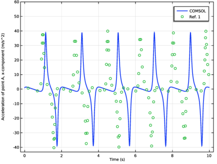
In the Settings window for Point Graph, click Replace Expression in the upper-right corner of the y-Axis Data section. From the menu, choose Component 1 (comp1)>Multibody Dynamics>Acceleration and velocity>Acceleration - m/s²>mbd.u_ttX - Acceleration, X component.
3
Click to expand the Coloring and Style section. From the Width list, choose 2.
4
Click to expand the Legends section. Select the Show legends check box.
5
From the Legends list, choose Manual.
6
Table Graph 1
1
In the Model Builder window, right-click Acceleration: point A and choose Table Graph.
2
In the Settings window for Table Graph, locate the Coloring and Style section.
3
Find the Line style subsection. From the Line list, choose None.
4
Find the Line markers subsection. From the Marker list, choose Circle.
5
Click to expand the Legends section. Select the Show legends check box.
6
From the Legends list, choose Manual.
7
8
In the Acceleration: point A toolbar, click  Plot.
9
Click the  Zoom Extents button in the Graphics toolbar.
Acceleration: point A
1
In the Model Builder window, click Acceleration: point A.
2
In the Settings window for 1D Plot Group, locate the Axis section.
3
Select the Manual axis limits check box.
4
In the y maximum text field, type 60.
5
Click to expand the Title section. From the Title type list, choose None.
6
Locate the Plot Settings section.
7
Select the x-axis label check box. In the associated text field, type Time (s).
8
Select the y-axis label check box. In the associated text field, type Acceleration of point A, x-component (m/s^2).
9
In the Acceleration: point A toolbar, click  Plot.
Use the following instructions to plot the energy variation in the slider crank mechanism as shown in Figure 4.
Energy
1
In the Home toolbar, click  Add Plot Group and choose 1D Plot Group.
2
In the Settings window for 1D Plot Group, type Energy in the Label text field.
Global 1
1
Right-click Energy and choose Global.
2
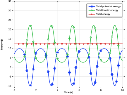
In the Settings window for Global, click Replace Expression in the upper-right corner of the y-Axis Data section. From the menu, choose Component 1 (comp1)>Definitions>Variables>Wp - Total potential energy - J.
3
Click Add Expression in the upper-right corner of the y-Axis Data section. From the menu, choose Component 1 (comp1)>Multibody Dynamics>Global>mbd.Wk_tot - Total kinetic energy - J.
4
Click Add Expression in the upper-right corner of the y-Axis Data section. From the menu, choose Component 1 (comp1)>Definitions>Variables>W - Total energy - J.
5
Click to expand the Coloring and Style section. From the Width list, choose 2.
6
Find the Line markers subsection. From the Marker list, choose Cycle.
7
From the Positioning list, choose Interpolated.
8
In the Number text field, type 24.
Energy
1
In the Model Builder window, click Energy.
2
In the Settings window for 1D Plot Group, locate the Axis section.
3
Select the Manual axis limits check box.
4
In the Energy toolbar, click  Plot.
5
Click the  Zoom Extents button in the Graphics toolbar.
6
In the y maximum text field, type 35.
7
Locate the Title section. From the Title type list, choose None.
8
Locate the Plot Settings section. Select the x-axis label check box.
9
Select the y-axis label check box. In the associated text field, type Energy (J).
10
In the Energy toolbar, click  Plot.
Finally, to generate an animation of the slider crank mechanism, follow these instructions:
Animation 1
1
In the Results toolbar, click  Animation and choose Player.
2
In the Settings window for Animation, locate the Frames section.
3
In the Number of frames text field, type 100.
4
Click the  Play button in the Graphics toolbar.