PDF

Assembly with a Hinge Joint
Introduction
In mechanical assemblies, parts are sometimes connected so that they are free to move relative to each other with one or multiple degrees of freedom. Examples of such connections are ball joints, hinges, and different types of bearings. If the details of the connection are not the subjects of the analysis, it is possible to model the connection using joint nodes in the Multibody Dynamics Module.
This example illustrates how to model a barrel hinge connecting two solid objects in an assembly. Two different versions are studied. In one of them, both parts are flexible. In the other version, one of the parts is considered as rigid.
Model Definition
Figure 1 shows the model geometry.
Figure 1: Model geometry.
Two parts of the assembly are connected through a barrel hinge that allows relative rotation as well as sliding along the axis of the pin hole. All the other degrees of freedom are shared between the two parts.
One hole of the forked bottom part is modeled as a hinge joint and other hole is modeled as a cylindrical joint allowing the axial motion.
The pin hole of the top part is constrained in the x direction so that it can slide in the y-plane.
A force of 1 kN is applied in z direction at a 10 cm distance in the negative y direction from the center of the upper pin hole. The offset of the load introduces both tension and bending of the member.
In a second study, the upper part is considered as rigid, and it only transmits the force through the hinge.
Results and Discussion
The default displacement plot for the flexible model is shown in Figure 2.
Figure 2: Displacement of the flexible structure.
In Figure 3 you can see the stress distribution.
Figure 3: Equivalent stress in the flexible structure
In a model that consists of a mix of rigid and flexible parts, stresses can only be displayed in the flexible parts. This is shown in Figure 4.
If you compare Figure 3 and Figure 4, you can see that the stress distribution in the lower part is essentially unaffected by the fact that the load is transmitted through a rigid body.
Figure 4: Equivalent stress in the flexible part when one component is rigid.
Notes About the COMSOL Implementation
When the flexibility of a component can be neglected and its stress distribution is not of interest, it is efficient to treat such a component as a rigid domain. The rigid domain is a domain that has a material model with only one material parameter, the density.
A Joint node can establish a connection directly between Rigid Material nodes however Attachment nodes are needed, defining the connection boundaries, for flexible elements.
Application Library path: Multibody_Dynamics_Module/Tutorials/hinge_joint_assembly
Modeling Instructions
From the File menu, choose New.
New
In the New window, click  Model Wizard.
Model Wizard
1
In the Model Wizard window, click  3D.
2
In the Select Physics tree, select Structural Mechanics>Multibody Dynamics (mbd).
3
Click Add.
4
Click  Study.
5
In the Select Study tree, select General Studies>Stationary.
6
Global Definitions
Parameters 1
1
In the Model Builder window, under Global Definitions click Parameters 1.
2
In the Settings window for Parameters, locate the Parameters section.
3
Geometry 1
Import 1 (imp1)
1
In the Home toolbar, click  Import.
2
In the Settings window for Import, locate the Import section.
3
Click  Browse.
4
5
Click  Import.
Form Union (fin)
1
In the Model Builder window, under Component 1 (comp1)>Geometry 1 click Form Union (fin).
2
In the Settings window for Form Union/Assembly, locate the Form Union/Assembly section.
3
From the Action list, choose Form an assembly.
4
Clear the Create pairs check box.
5
Click  Build Selected.
Add Material
1
In the Home toolbar, click  Add Material to open the Add Material window.
2
Go to the Add Material window.
3
In the tree, select Built-in>Structural steel.
4
Click Add to Component in the window toolbar.
5
In the Home toolbar, click  Add Material to close the Add Material window.
Multibody Dynamics (mbd)
Fixed Constraint 1
1
In the Model Builder window, under Component 1 (comp1) right-click Multibody Dynamics (mbd) and choose Fixed Constraint.
2
Use Rigid Connector node to constrain the motion and apply load.
Rigid Connector 1
1
In the Physics toolbar, click  Boundaries and choose Rigid Connector.
2
3
In the Settings window for Rigid Connector, locate the Prescribed Displacement at Center of Rotation section.
4
Select the Prescribed in x direction check box.
Applied Force 1
1
In the Physics toolbar, click  Attributes and choose Applied Force.
2
In the Settings window for Applied Force, locate the Location section.
3
Select the Offset check box.
4
Specify the Xoffset vector as
The center of rotation for a rigid connector is available in the variables xcx_tag, xcy_tag, and xcz_tag. The default position is the center of gravity of the attached boundaries, which in this case will be the center of the hole.
5
Locate the Applied Force section. Specify the F vector as
Attachment 1
1
In the Physics toolbar, click  Boundaries and choose Attachment.
2
3
In the Settings window for Attachment, locate the Connection Type section.
4
Attachment 2
1
In the Physics toolbar, click  Boundaries and choose Attachment.
2
3
In the Settings window for Attachment, locate the Connection Type section.
4
Attachment 3
1
In the Physics toolbar, click  Boundaries and choose Attachment.
2
3
In the Settings window for Attachment, locate the Connection Type section.
4
Hinge Joint 1
1
In the Physics toolbar, click  Global and choose Hinge Joint.
2
In the Settings window for Hinge Joint, locate the Attachment Selection section.
3
From the Source list, choose Attachment 1.
4
From the Destination list, choose Attachment 3.
5
Locate the Axis of Joint section. Specify the e0 vector as
Cylindrical Joint 1
1
In the Physics toolbar, click  Global and choose Cylindrical Joint.
2
In the Settings window for Cylindrical Joint, locate the Attachment Selection section.
3
From the Source list, choose Attachment 2.
4
From the Destination list, choose Attachment 3.
5
Locate the Axis of Joint section. Specify the e0 vector as
If you want accurate stress results, then quadratic shape functions should be used for the displacements. The default value in the Multibody Dynamics interface is linear shape functions.
6
In the Model Builder window, click Multibody Dynamics (mbd).
7
In the Settings window for Multibody Dynamics, click to expand the Discretization section.
8
From the Displacement field list, choose Quadratic Lagrange.
Mesh 1
Free Tetrahedral 1
In the Mesh toolbar, click  Free Tetrahedral.
Size 1
1
Right-click Free Tetrahedral 1 and choose Size.
2
In the Settings window for Size, locate the Geometric Entity Selection section.
3
From the Geometric entity level list, choose Boundary.
4
5
Locate the Element Size section. Click the Custom button.
6
Locate the Element Size Parameters section.
7
Select the Maximum element size check box. In the associated text field, type 0.002.
Size
1
In the Model Builder window, under Component 1 (comp1)>Mesh 1 click Size.
2
In the Settings window for Size, locate the Element Size section.
3
From the Predefined list, choose Fine.
4
Click  Build All.
Study 1
In the Home toolbar, click  Compute.
Results
Displacement (mbd)
1
In the Displacement (mbd) toolbar, click  Plot.
The default plot shows the displacement of the assembly. Compare with Figure 2.
Reproduce the stress plot shown in Figure 3 with the following steps.
Stress
1
In the Home toolbar, click  Add Plot Group and choose 3D Plot Group.
2
In the Settings window for 3D Plot Group, type Stress in the Label text field.
Surface 1
1
Right-click Stress and choose Surface.
2
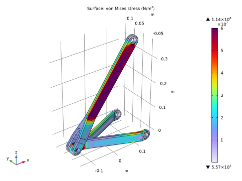
In the Settings window for Surface, click Replace Expression in the upper-right corner of the Expression section. From the menu, choose Component 1 (comp1)>Multibody Dynamics>Stress>mbd.mises - von Mises stress - N/m².
3
In the Stress toolbar, click  Plot.
4
Click to expand the Range section. Select the Manual color range check box.
5
In the Maximum text field, type 6E7.
6
Locate the Coloring and Style section. Click  Change Color Table.
7
In the Color Table dialog box, select Rainbow>Prism in the tree.
8
Stress
1
In the Model Builder window, click Stress.
2
In the Settings window for 3D Plot Group, locate the Color Legend section.
3
Select the Show maximum and minimum values check box.
4
In the Stress toolbar, click  Plot.
Make the upper lever rigid and analyze that configuration in a new study.
Multibody Dynamics (mbd)
Rigid Material 1
1
In the Physics toolbar, click  Domains and choose Rigid Material.
2
Use Rigid Material subnodes to constrain the motion and apply load.
Prescribed Displacement/Rotation 1
1
In the Physics toolbar, click  Attributes and choose Prescribed Displacement/Rotation.
2
In the Settings window for Prescribed Displacement/Rotation, locate the Prescribed Displacement at Center of Rotation section.
3
Select the Prescribed in x direction check box.
4
Locate the Center of Rotation section. From the list, choose Centroid of selected entities.
Center of Rotation: Boundary 1
1
In the Model Builder window, expand the Prescribed Displacement/Rotation 1 node, then click Center of Rotation: Boundary 1.
2
Rigid Material 1
In the Model Builder window, under Component 1 (comp1)>Multibody Dynamics (mbd) click Rigid Material 1.
Applied Force 1
1
In the Physics toolbar, click  Attributes and choose Applied Force.
Similar to the previous case, point of load application can be written like as follows:
2
In the Settings window for Applied Force, locate the Location section.
3
4
Specify the Xp vector as
5
Locate the Applied Force section. Specify the F vector as
Add an extra Hinge Joint node, so that it is easy to rerun the original version of the model. Normally it would have been easier just to utilize the existing joint.
Add Study
1
In the Home toolbar, click  Add Study to open the Add Study window.
2
Go to the Add Study window.
3
Find the Studies subsection. In the Select Study tree, select General Studies>Stationary.
4
Click Add Study in the window toolbar.
5
In the Home toolbar, click  Add Study to close the Add Study window.
Study 2
In the Home toolbar, click  Compute.
Results
Stress
Duplicate the stress plot used for the fully flexible model to get Figure 4.
Stress 1
1
In the Model Builder window, right-click Stress and choose Duplicate.
2
In the Settings window for 3D Plot Group, locate the Data section.
3
From the Dataset list, choose Study 2/Solution 2 (sol2).
4
In the Stress 1 toolbar, click  Plot.
Make sure that the first study still solves for the flexible structure.
Study 1
Step 1: Stationary
1
In the Model Builder window, under Study 1 click Step 1: Stationary.
2
In the Settings window for Stationary, locate the Physics and Variables Selection section.
3
Select the Modify model configuration for study step check box.
4
In the tree, select Component 1 (comp1)>Multibody Dynamics (mbd), Controls spatial frame>Rigid Material 1.
5
Click  Disable.