
|
|
|
|
•
|
Case-1: Basic hinge joint
|
|
•
|
Case-2: Constraints on joint
|
|
•
|
Case-3: Locking on joint
|
|
•
|
Case-4: Spring and damper on joint
|
|
•
|
Case-5: Prescribed motion on joint
|
|
•
|
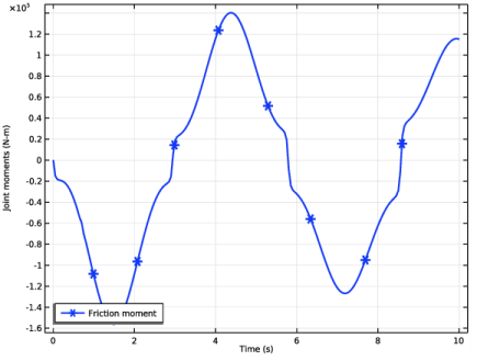
Case-6: Friction on joint
|
|
•
|
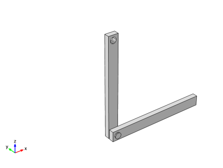
For the first three cases, both arms are modeled as flexible elements using the Linear Elastic Material model, and in the last three cases they are modeled as rigid elements using the Rigid Material model. Rigid elements can be used if the stresses and the deformation in the components are of no interest.
|
|
•
|
A Joint node can directly establish a connection between Rigid Material nodes. However, in flexible elements, Attachment nodes are needed to define the connection boundaries.
|
|
•
|
Constraint boundary conditions, like Rigid Connector and Fixed Constraint, cannot be used with the Rigid Material node. Hence, the Prescribed Displacement/Rotation node (subnode of Rigid Material) is used to prescribe the degrees of freedom.
|

|
1
|
|
2
|
|
3
|
Click Add.
|
|
4
|
Click
|
|
5
|
|
6
|
Click
|
|
1
|
|
2
|
|
3
|
|
4
|
|
1
|
|
2
|
|
3
|
|
4
|
|
5
|
|
6
|
|
7
|
|
1
|
|
2
|
Select the object blk1 only.
|
|
3
|
|
4
|
|
5
|
Select the object cyl1 only.
|
|
1
|
|
2
|
|
3
|
|
4
|
|
5
|
|
6
|
|
7
|
|
8
|
|
1
|
|
2
|
Select the object cyl2 only.
|
|
1
|
|
2
|
|
3
|
|
4
|
|
5
|
|
1
|
|
2
|
Select the object blk2 only.
|
|
3
|
|
4
|
|
5
|
Select the object copy1 only.
|
|
1
|
|
2
|
|
3
|
|
4
|
|
1
|
|
2
|
|
3
|
|
4
|
|
1
|
|
2
|
Click in the Graphics window and then press Ctrl+A to select both domains.
|
|
1
|
|
2
|
|
1
|
|
2
|
|
3
|
|
4
|
|
5
|
|
1
|
|
1
|
|
2
|
|
3
|
|
4
|
|
5
|
|
6
|
|
1
|
|
1
|
|
1
|
|
2
|
|
3
|
|
4
|
|
5
|
|
1
|
|
2
|
|
3
|
|
4
|
|
5
|
|
6
|
|
1
|
|
3
|
|
4
|
|
1
|
|
2
|
|
3
|
|
4
|
|
5
|
|
1
|
|
2
|
|
1
|
|
2
|
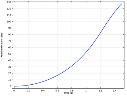
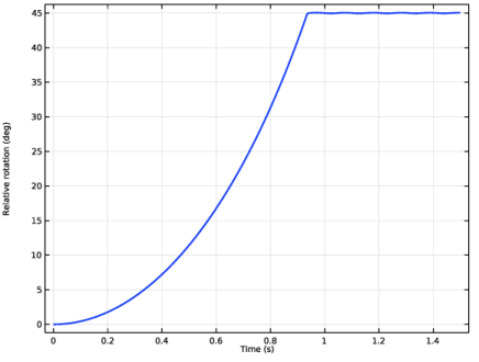
In the Settings window for Global, click Replace Expression in the upper-right corner of the y-Axis Data section. From the menu, choose Component 1 (comp1)>Multibody Dynamics>Hinge joints>Hinge Joint 2>mbd.hgj2.th - Relative rotation - rad.
|
|
3
|
|
4
|
|
5
|
|
6
|
|
7
|
|
1
|
|
2
|
|
1
|
|
2
|
In the Settings window for Global, click Replace Expression in the upper-right corner of the y-Axis Data section. From the menu, choose Component 1 (comp1)>Multibody Dynamics>Hinge joints>Hinge Joint 2>Joint force - N>mbd.hgj2.Fx - Joint force, x component.
|
|
3
|
Click Add Expression in the upper-right corner of the y-Axis Data section. From the menu, choose Component 1 (comp1)>Multibody Dynamics>Hinge joints>Hinge Joint 2>Joint force - N>mbd.hgj2.Fy - Joint force, y component.
|
|
4
|
Click Add Expression in the upper-right corner of the y-Axis Data section. From the menu, choose Component 1 (comp1)>Multibody Dynamics>Hinge joints>Hinge Joint 2>Joint force - N>mbd.hgj2.Fz - Joint force, z component.
|
|
5
|
|
6
|
|
7
|
|
8
|
|
1
|
|
2
|
|
3
|
|
4
|
|
5
|
|
1
|
In the Model Builder window, under Component 1 (comp1)>Multibody Dynamics (mbd) click Hinge Joint 2.
|
|
2
|
|
3
|
|
4
|
|
5
|
|
6
|
|
1
|
|
2
|
|
3
|
|
1
|
|
2
|
|
3
|
|
4
|
|
5
|
|
1
|
|
2
|
|
3
|
|
4
|
|
5
|
|
6
|
|
1
|
|
2
|
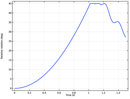
In the Settings window for 1D Plot Group, type Relative rotation: Constraints in the Label text field.
|
|
3
|
|
4
|
|
1
|
|
2
|
|
3
|
|
1
|
|
2
|
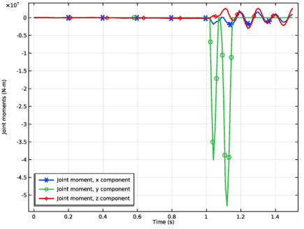
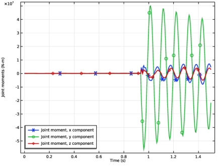
In the Settings window for Global, click Replace Expression in the upper-right corner of the y-Axis Data section. From the menu, choose Component 1 (comp1)>Multibody Dynamics>Hinge joints>Hinge Joint 2>Joint moment - N·m>mbd.hgj2.Mx - Joint moment, x component.
|
|
3
|
Click Add Expression in the upper-right corner of the y-Axis Data section. From the menu, choose Component 1 (comp1)>Multibody Dynamics>Hinge joints>Hinge Joint 2>Joint moment - N·m>mbd.hgj2.My - Joint moment, y component.
|
|
4
|
Click Add Expression in the upper-right corner of the y-Axis Data section. From the menu, choose Component 1 (comp1)>Multibody Dynamics>Hinge joints>Hinge Joint 2>Joint moment - N·m>mbd.hgj2.Mz - Joint moment, z component.
|
|
1
|
|
2
|
|
3
|
|
4
|
|
5
|
|
1
|
|
2
|
|
1
|
|
2
|
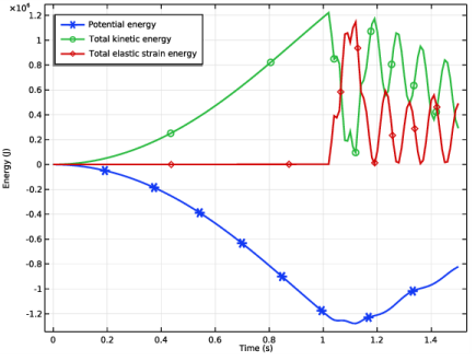
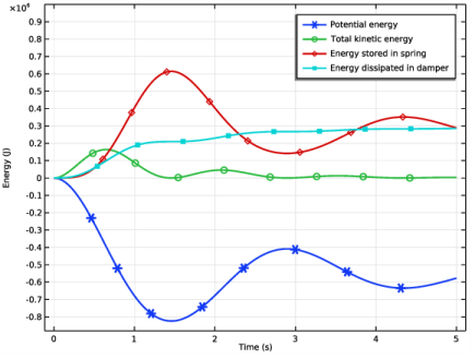
In the Settings window for Global, click Replace Expression in the upper-right corner of the y-Axis Data section. From the menu, choose Component 1 (comp1)>Definitions>Variables>Wp - Potential energy - J.
|
|
3
|
Click Add Expression in the upper-right corner of the y-Axis Data section. From the menu, choose Component 1 (comp1)>Multibody Dynamics>Global>mbd.Wk_tot - Total kinetic energy - J.
|
|
4
|
Click Add Expression in the upper-right corner of the y-Axis Data section. From the menu, choose Component 1 (comp1)>Multibody Dynamics>Global>mbd.Ws_tot - Total elastic strain energy - J.
|
|
1
|
|
2
|
|
3
|
|
4
|
|
5
|
|
1
|
In the Model Builder window, under Component 1 (comp1)>Multibody Dynamics (mbd) click Hinge Joint 2.
|
|
2
|
|
3
|
|
1
|
|
1
|
|
2
|
|
3
|
|
4
|
|
1
|
|
1
|
|
2
|
|
3
|
|
1
|
|
2
|
|
3
|
|
4
|
|
5
|
|
1
|
|
2
|
|
3
|
Locate the Physics and Variables Selection section. Select the Modify model configuration for study step check box.
|
|
4
|
In the tree, select Component 1 (comp1)>Multibody Dynamics (mbd), Controls spatial frame>Hinge Joint 1>Prescribed Motion 1 and Component 1 (comp1)>Multibody Dynamics (mbd), Controls spatial frame>Hinge Joint 2>Constraints 1.
|
|
5
|
Right-click and choose Disable.
|
|
6
|
|
7
|
|
8
|
|
1
|
|
2
|
|
3
|
|
4
|
|
5
|
In the Model Builder window, expand the Study: Locking>Solver Configurations>Solution 3 (sol3)>Time-Dependent Solver 1 node, then click Fully Coupled 1.
|
|
6
|
|
7
|
|
8
|
|
1
|
|
2
|
|
3
|
|
4
|
|
1
|
|
2
|
|
3
|
|
4
|
|
1
|
|
1
|
|
1
|
|
2
|
|
3
|
|
4
|
|
5
|
|
6
|
|
7
|
|
1
|
|
2
|
|
3
|
|
4
|
|
5
|
|
6
|
In the Show More Options dialog box, in the tree, select the check box for the node Physics>Equation-Based Contributions.
|
|
7
|
Click OK.
|
|
1
|
|
2
|
|
3
|
|
4
|
|
5
|
|
6
|
Click
|
|
7
|
|
8
|
Click OK.
|
|
9
|
|
10
|
|
11
|
|
12
|
Click
|
|
13
|
|
14
|
Click OK.
|
|
1
|
|
2
|
|
3
|
|
4
|
|
5
|
|
1
|
|
2
|
|
3
|
Locate the Physics and Variables Selection section. Select the Modify model configuration for study step check box.
|
|
4
|
In the tree, select Component 1 (comp1)>Multibody Dynamics (mbd), Controls spatial frame>Hinge Joint 1.
|
|
5
|
Right-click and choose Disable.
|
|
6
|
In the tree, select Component 1 (comp1)>Multibody Dynamics (mbd), Controls spatial frame>Attachment 1, Component 1 (comp1)>Multibody Dynamics (mbd), Controls spatial frame>Attachment 2, and Component 1 (comp1)>Multibody Dynamics (mbd), Controls spatial frame>Attachment 3.
|
|
7
|
Right-click and choose Disable.
|
|
8
|
In the tree, select Component 1 (comp1)>Multibody Dynamics (mbd), Controls spatial frame>Hinge Joint 2.
|
|
9
|
Right-click and choose Disable.
|
|
10
|
|
11
|
|
12
|
|
13
|
|
1
|
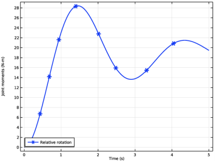
In the Settings window for 1D Plot Group, type Relative rotation: Spring-Damper in the Label text field.
|
|
2
|
|
1
|
|
2
|
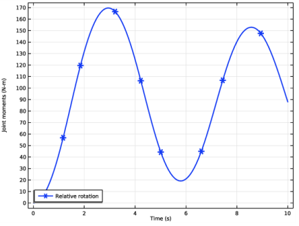
In the Settings window for Global, click Replace Expression in the upper-right corner of the y-Axis Data section. From the menu, choose Component 1 (comp1)>Multibody Dynamics>Hinge joints>Hinge Joint 3>comp1.mbd.hgj3.th - Relative rotation - rad.
|
|
3
|
|
1
|
|
2
|
|
3
|
|
4
|
|
1
|
|
2
|
|
3
|
|
1
|
|
2
|
In the Settings window for Global, click Replace Expression in the upper-right corner of the y-Axis Data section. From the menu, choose Component 1 (comp1)>Definitions>Variables>Wp - Potential energy - J.
|
|
3
|
Click Add Expression in the upper-right corner of the y-Axis Data section. From the menu, choose Component 1 (comp1)>Multibody Dynamics>Global>mbd.Wk_tot - Total kinetic energy - J.
|
|
4
|
|
5
|
|
6
|
|
7
|
|
8
|
|
1
|
|
2
|
|
3
|
|
4
|
|
5
|
|
6
|
|
7
|
|
1
|
|
2
|
|
3
|
|
4
|
|
5
|
|
6
|
|
1
|
|
2
|
|
3
|
|
4
|
|
5
|
|
1
|
|
2
|
|
3
|
Locate the Physics and Variables Selection section. Select the Modify model configuration for study step check box.
|
|
4
|
In the tree, select Component 1 (comp1)>Multibody Dynamics (mbd), Controls spatial frame>Gravity 1, Component 1 (comp1)>Multibody Dynamics (mbd), Controls spatial frame>Attachment 1, Component 1 (comp1)>Multibody Dynamics (mbd), Controls spatial frame>Hinge Joint 1, Component 1 (comp1)>Multibody Dynamics (mbd), Controls spatial frame>Attachment 2, Component 1 (comp1)>Multibody Dynamics (mbd), Controls spatial frame>Attachment 3, Component 1 (comp1)>Multibody Dynamics (mbd), Controls spatial frame>Hinge Joint 2, Component 1 (comp1)>Multibody Dynamics (mbd), Controls spatial frame>Hinge Joint 3>Spring and Damper 1, and Component 1 (comp1)>Multibody Dynamics (mbd), Controls spatial frame>Energy: Damper.
|
|
5
|
Right-click and choose Disable.
|
|
6
|
|
7
|
|
8
|
|
9
|
|
1
|
|
2
|
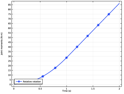
In the Settings window for 1D Plot Group, type Relative rotation: Prescribed motion in the Label text field.
|
|
3
|
|
4
|
|
1
|
|
2
|
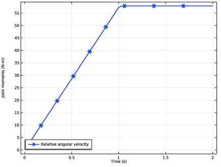
In the Settings window for 1D Plot Group, type Relative velocity: Prescribed motion in the Label text field.
|
|
3
|
|
1
|
In the Model Builder window, expand the Relative velocity: Prescribed motion node, then click Global 1.
|
|
2
|
In the Settings window for Global, click Replace Expression in the upper-right corner of the y-Axis Data section. From the menu, choose Component 1 (comp1)>Multibody Dynamics>Hinge joints>Hinge Joint 3>mbd.hgj3.th_t - Relative angular velocity - rad/s.
|
|
3
|
|
1
|
|
2
|
|
1
|
In the Model Builder window, under Component 1 (comp1)>Multibody Dynamics (mbd) click Hinge Joint 3.
|
|
2
|
|
3
|
|
1
|
|
2
|
|
3
|
|
4
|
|
1
|
|
2
|
|
3
|
|
1
|
|
2
|
|
3
|
|
4
|
|
5
|
|
1
|
|
2
|
|
3
|
Locate the Physics and Variables Selection section. Select the Modify model configuration for study step check box.
|
|
4
|
In the tree, select Component 1 (comp1)>Multibody Dynamics (mbd), Controls spatial frame>Attachment 1, Component 1 (comp1)>Multibody Dynamics (mbd), Controls spatial frame>Hinge Joint 1, Component 1 (comp1)>Multibody Dynamics (mbd), Controls spatial frame>Attachment 2, Component 1 (comp1)>Multibody Dynamics (mbd), Controls spatial frame>Attachment 3, Component 1 (comp1)>Multibody Dynamics (mbd), Controls spatial frame>Hinge Joint 2, Component 1 (comp1)>Multibody Dynamics (mbd), Controls spatial frame>Hinge Joint 3>Spring and Damper 1, Component 1 (comp1)>Multibody Dynamics (mbd), Controls spatial frame>Hinge Joint 3>Prescribed Motion 1, and Component 1 (comp1)>Multibody Dynamics (mbd), Controls spatial frame>Energy: Damper.
|
|
5
|
Right-click and choose Disable.
|
|
6
|
|
7
|
|
8
|
|
1
|
|
2
|
|
3
|
In the Model Builder window, expand the Study: Friction>Solver Configurations>Solution 6 (sol6)>Dependent Variables 1 node, then click Energy loss due to friction (comp1.ODE1).
|
|
4
|
|
5
|
|
6
|
|
7
|
|
1
|
|
2
|
|
3
|
|
4
|
|
1
|
|
2
|
|
1
|
|
2
|
|
1
|
|
2
|
|
1
|
|
2
|
|
3
|
|
4
|
|
5
|
|
1
|
|
2
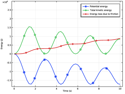
|
In the Settings window for Global, click Replace Expression in the upper-right corner of the y-Axis Data section. From the menu, choose Component 1 (comp1)>Definitions>Variables>Wp - Potential energy - J.
|
|
3
|
Click Add Expression in the upper-right corner of the y-Axis Data section. From the menu, choose Component 1 (comp1)>Multibody Dynamics>Global>mbd.Wk_tot - Total kinetic energy - J.
|
|
4
|
|
5
|
|
6
|
|
7
|
|
8
|
|
1
|
|
2
|
|
3
|
|
4
|
|
5
|
|
6
|
|
7
|
|
1
|
|
2
|
|
3
|
|
4
|
|
1
|
|
2
|
|
3
|
In the tree, select Component 1 (comp1)>Multibody Dynamics (mbd), Controls spatial frame>Hinge Joint 3>Friction 1 and Component 1 (comp1)>Multibody Dynamics (mbd), Controls spatial frame>Energy: Friction.
|
|
4
|
Right-click and choose Disable.
|
|
1
|
|
2
|
|
3
|
In the tree, select Component 1 (comp1)>Multibody Dynamics (mbd), Controls spatial frame>Hinge Joint 3>Prescribed Motion 1, Component 1 (comp1)>Multibody Dynamics (mbd), Controls spatial frame>Hinge Joint 3>Friction 1, and Component 1 (comp1)>Multibody Dynamics (mbd), Controls spatial frame>Energy: Friction.
|
|
4
|
Right-click and choose Disable.
|
|
1
|
|
2
|
|
3
|
In the tree, select Component 1 (comp1)>Multibody Dynamics (mbd), Controls spatial frame>Rigid Material 1, Component 1 (comp1)>Multibody Dynamics (mbd), Controls spatial frame>Rigid Material 2, Component 1 (comp1)>Multibody Dynamics (mbd), Controls spatial frame>Hinge Joint 3, Component 1 (comp1)>Multibody Dynamics (mbd), Controls spatial frame>Energy: Damper, and Component 1 (comp1)>Multibody Dynamics (mbd), Controls spatial frame>Energy: Friction.
|
|
4
|
Right-click and choose Disable.
|
|
1
|
|
2
|
|
3
|
|
4
|
In the tree, select Component 1 (comp1)>Multibody Dynamics (mbd), Controls spatial frame>Hinge Joint 2>Locking 1, Component 1 (comp1)>Multibody Dynamics (mbd), Controls spatial frame>Rigid Material 1, Component 1 (comp1)>Multibody Dynamics (mbd), Controls spatial frame>Rigid Material 2, Component 1 (comp1)>Multibody Dynamics (mbd), Controls spatial frame>Hinge Joint 3, Component 1 (comp1)>Multibody Dynamics (mbd), Controls spatial frame>Energy: Damper, and Component 1 (comp1)>Multibody Dynamics (mbd), Controls spatial frame>Energy: Friction.
|
|
5
|
Right-click and choose Disable.
|
|
1
|
|
2
|
|
3
|
|
4
|
In the tree, select Component 1 (comp1)>Multibody Dynamics (mbd), Controls spatial frame>Hinge Joint 1>Prescribed Motion 1, Component 1 (comp1)>Multibody Dynamics (mbd), Controls spatial frame>Hinge Joint 2>Constraints 1, Component 1 (comp1)>Multibody Dynamics (mbd), Controls spatial frame>Hinge Joint 2>Locking 1, Component 1 (comp1)>Multibody Dynamics (mbd), Controls spatial frame>Rigid Material 1, Component 1 (comp1)>Multibody Dynamics (mbd), Controls spatial frame>Rigid Material 2, Component 1 (comp1)>Multibody Dynamics (mbd), Controls spatial frame>Hinge Joint 3, Component 1 (comp1)>Multibody Dynamics (mbd), Controls spatial frame>Energy: Damper, and Component 1 (comp1)>Multibody Dynamics (mbd), Controls spatial frame>Energy: Friction.
|
|
5
|
Right-click and choose Disable.
|