PDF

Thermo-Photo-Voltaic Cell
Introduction
The following example illustrates an application that maximizes surface-to-surface radiative fluxes and minimizes conductive heat fluxes.
A thermo-photo-voltaic (TPV) cell generates electricity from the combustion of fuel and through radiation. Figure 1 depicts the general operating principle. The fuel burns inside an emitting device that radiates intensely. Photovoltaic (PV) cells — almost like solar cells — capture the radiation and convert it to electricity. The efficiency of a TPV device ranges from 1% to 20%. In some cases, TPVs are used in heat generators to co-generate electricity, and the efficiency is not so critical. In other cases TPVs are used as electric power sources, for example in automobiles (Ref. 1). In those cases efficiency is a major concern.
Figure 1: Operating principle of a TPV device (Ref. 2), and an image of a prototype system (Ref. 3).
TPV systems, unlike typical electronic systems, must maximize radiation heat transfer to improve efficiency. However, inherent radiation losses — radiation not converted to electric power — contributes to the PV cells’ increased temperature. Further, heat transfer through conduction results in increased cell temperature. PV cells have a limited operating temperature range that depends on the type of material used. Solar cells are limited to temperatures below 80°C, whereas high-efficiency semiconductor materials can withstand as much as 1000°C. Photovoltaic efficiency is often a function of temperature with a maximum at some temperature above ambient.
To improve system efficiency, engineers prefer to use high-efficiency PV cells, which however can be quite expensive. To reduce system costs, engineers work with smaller-area PV cells and then use mirrors to focus the radiation on them. However, there is a limit for how much you can focus the beams; if the radiation intensity becomes too high, the cells can overheat. Thus engineers must optimize system geometry and operating conditions to achieve maximum performance at minimum material costs.
The following application, which uses the Heat Transfer with Surface-to-Surface Radiation interface, investigates the influence of operating conditions (flame temperature) on system efficiency and the temperature of components in a typical TPV system. The application can also assess the influence of geometry changes.
Model Definition
Figure 2 depicts the geometry and dimensions of the system under study. To reduce the temperature, the PV cells are water cooled on their back side (at the interface with the insulation).
Figure 2: Geometry and dimensions of the modeled TPV system.
Conduction is always present on the different boundaries. The model simulates the emitter with a specific temperature, Theater, on the inner boundary. At the outer emitter boundary, it takes radiation (surface-to-surface) into account in the boundary condition. It simulates the mirrors by taking radiation into account on all boundaries and applying a low emissivity. The inner boundaries of the PV cells and of the insulation also make use of radiation boundary conditions. However, the PV cells have a high emissivity and the insulation a low emissivity. Further, the PV cells convert a fraction of the irradiation to electricity instead of heat. Heat sinks on their inner boundaries simulate this effect by accounting for a boundary heat source, q, defined by
where G is the irradiation flux (W/m2) and ηpv is the PV cell’s voltaic efficiency. The latter depends on the local temperature, with a maximum of 0.2 at 800 K:
Figure 3 illustrates this expression for temperatures above 1000 K.
Figure 3: PV cell voltaic efficiency versus temperature.
At the outer boundary of the PV cells, the model applies convective water cooling by setting h to 50 W/(m2·K), and Tamb to 273.15 K. Finally, at the outer boundary of the insulation it applies convective cooling with h set to 5 W/(m2·K) and Tamb to 293.15 K.
Table 1 summarizes the material properties.
k (W/(m·K))
ρ (kg/m3)
Cp (J/(kg·K))
ε
The model calculates the stationary solution for a range of emitter temperatures (1000 K to 2000 K) using the parametric solver.
Finally, the geometry shown in Figure 2 allows taking advantage of sector symmetry and reflection to reduce the computational cost. As shown in Figure 4, the geometry can be divided in 8 sectors (delimited by blue lines), each containing a reflection plane (red line). The computational domain is thus reduced to one sixteenth of the geometry. Then, for surface-to-surface radiation modeling, the view factor computation on the reduced geometry takes into account the presence of all the surfaces of the full geometry.
Figure 4: Sectors of symmetry (blue lines) and reflection plane (red line) in one sector.
Results and Discussion
The results shows that the device experiences a significant temperature distribution that varies with operating conditions. Figure 5 depicts the stationary distribution on full geometry at operating conditions with an emitter temperature of 2000 K.
Figure 5: Temperature distribution in the TPV system when the emitter temperature is 2000 K.
As the upper plot in Figure 6 shows, the PV cells reach a temperature of approximately 1800 K. This is significantly higher than their maximum operating temperature of 1600 K, above which their photovoltaic efficiency is zero (see Figure 3).
It is interesting to investigate what the optimal operating temperature is. The lower plot in Figure 6 investigates at what temperature the system achieves the maximum electric power output. The optimal emitter temperature for this configuration seems to be between 1600 K and 1700 K, where the electric power (irradiation multiplied by voltaic efficiency) is maximum.
Figure 6: PV cell temperature (top) and electric output power (bottom) versus operating temperature.
The next step is to look at the temperature distribution at the optimal operating conditions (Figure 7).
Figure 7: Temperature distribution and surface irradiation flux in the system at an operating emitter temperature of 1600 K.
When the emitter is at 1600 K, the PV cells reach a temperature of approximately 1200 K, which they can withstand without any problems. Note that the insulation reaches a temperature of approximately 800 K on the outside, suggesting that the system transfers a significant amount of heat to the surrounding air.
The irradiative flux varies significantly along the circumference of the PV cell and insulation jacket. To further investigate this effect, Figure 8 plots the irradiative flux at this operating condition in one sector of symmetry. Clearly the variation it shows is related to the positions of the mirrors and is an effect of shadowing.
Figure 8: Irradiation flux along the TPV cells, insulation inner surface at an operating emitter temperature of 1600 K.
This plot can help optimize the mirror geometry as well as help decide how large the PV cells should be and where they should be placed.
A general conclusion is that this type of modeling can shortcut the prototype development time and optimize the operating conditions for the finalized TPV device.
References
1. S. Christ and M. Seal, “Viking 27 — A Thermophotovoltaic Hybrid Vehicle Designed and Built at Western Washington University”, SAE Technical Paper 972650, 1997.
2. Courtesy of E. Fontes, Catella Generics AB, Sweden.
3. Courtesy of Dr. D. Wilhelm, Paul Sherrer Institute, Switzerland.
Application Library path: Heat_Transfer_Module/Thermal_Radiation/tpv_cell
Modeling Instructions
From the File menu, choose New.
New
In the New window, click  Model Wizard.
Model Wizard
1
In the Model Wizard window, click  2D.
2
In the Select Physics tree, select Heat Transfer>Radiation>Heat Transfer with Surface-to-Surface Radiation.
3
Click Add.
4
Click  Study.
5
In the Select Study tree, select General Studies>Stationary.
6
Global Definitions
Parameters 1
1
In the Model Builder window, under Global Definitions click Parameters 1.
2
In the Settings window for Parameters, locate the Parameters section.
3
Geometry 1
1
In the Model Builder window, under Component 1 (comp1) click Geometry 1.
2
In the Settings window for Geometry, locate the Units section.
3
From the Length unit list, choose mm.
Circle 1 (c1)
1
In the Geometry toolbar, click  Circle.
2
In the Settings window for Circle, locate the Size and Shape section.
3
In the Radius text field, type 40.
4
In the Sector angle text field, type 360/16.
5
Click to expand the Layers section. In the table, enter the following settings:
6
Click  Build Selected.
Rectangle 1 (r1)
1
In the Geometry toolbar, click  Rectangle.
2
In the Settings window for Rectangle, locate the Size and Shape section.
3
In the Width text field, type 2.
4
In the Height text field, type 5.
5
Locate the Position section. In the x text field, type 20.
6
Click  Build Selected.
Rectangle 2 (r2)
1
In the Geometry toolbar, click  Rectangle.
2
In the Settings window for Rectangle, locate the Size and Shape section.
3
In the Width text field, type 6.
4
Locate the Position section. In the x text field, type 20.
5
Click  Build Selected.
Union 1 (uni1)
1
In the Geometry toolbar, click  Booleans and Partitions and choose Union.
2
Select the objects r1 and r2 only.
3
In the Settings window for Union, locate the Union section.
4
Clear the Keep interior boundaries check box.
5
Click  Build Selected.
Fillet 1 (fil1)
1
In the Geometry toolbar, click  Fillet.
2
On the object uni1, select Points 3, 6, and 8 only.
It might be easier to select the correct points by using the Selection List window. To open this window, in the Home toolbar click Windows and choose Selection List. (If you are running the cross-platform desktop, you find Windows in the main menu.)
3
In the Settings window for Fillet, locate the Radius section.
4
In the Radius text field, type 0.5.
5
Click  Build Selected.
Circle 2 (c2)
1
In the Geometry toolbar, click  Circle.
2
In the Settings window for Circle, locate the Size and Shape section.
3
In the Radius text field, type 37.
4
In the Sector angle text field, type 360/48.
5
Locate the Rotation Angle section. In the Rotation text field, type 360/24.
6
Locate the Layers section. In the table, enter the following settings:
7
Click  Build Selected.
Delete Entities 1 (del1)
1
In the Model Builder window, right-click Geometry 1 and choose Delete Entities.
2
In the Settings window for Delete Entities, locate the Entities or Objects to Delete section.
3
From the Geometric entity level list, choose Domain.
4
On the object c2, select Domain 1 only.
5
In the Geometry toolbar, click  Build All.
6
Click the  Zoom Extents button in the Graphics toolbar.
The model geometry is now complete. It represents one sixteenth of the full geometry by taking advantage of the sector symmetry and reflection plane within each sector.
Materials
Insulation
1
In the Materials toolbar, click  Blank Material.
2
In the Settings window for Material, type Insulation in the Label text field.
3
Locate the Material Contents section. In the table, enter the following settings:
PV Cell
1
In the Materials toolbar, click  Blank Material.
2
In the Settings window for Material, type PV Cell in the Label text field.
3
This is the PV-cell domain.
4
Locate the Material Contents section. In the table, enter the following settings:
Mirror
1
In the Materials toolbar, click  Blank Material.
2
In the Settings window for Material, type Mirror in the Label text field.
3
4
Locate the Material Contents section. In the table, enter the following settings:
Emitter
1
In the Materials toolbar, click  Blank Material.
2
In the Settings window for Material, type Emitter in the Label text field.
3
4
Locate the Material Contents section. In the table, enter the following settings:
Add Material
1
In the Materials toolbar, click  Add Material to open the Add Material window.
2
Go to the Add Material window.
3
4
Click Add to Component in the window toolbar.
5
In the Materials toolbar, click  Add Material to close the Add Material window.
Materials
Air (mat5)
Select Domains 1 and 3 only.
Heat Transfer in Solids (ht)
Fluid 1
1
In the Model Builder window, under Component 1 (comp1) right-click Heat Transfer in Solids (ht) and choose Fluid.
2
3
In the Settings window for Fluid, locate the Thermodynamics, Fluid section.
4
From the Fluid type list, choose Gas/Liquid.
5
From the γ list, choose User defined.
Heat Flux 1
1
In the Physics toolbar, click  Boundaries and choose Heat Flux.
2
This is the outer boundary of the modeling domain, where convective air cooling is applied.
3
In the Settings window for Heat Flux, locate the Heat Flux section.
4
From the Flux type list, choose Convective heat flux.
5
In the h text field, type 5.
Boundary Heat Source 1
1
In the Physics toolbar, click  Boundaries and choose Boundary Heat Source.
2
These are the outward-facing PV-cell boundaries.
3
In the Settings window for Boundary Heat Source, locate the Boundary Heat Source section.
4
In the Qb text field, type 50[W/(m^2*K)]*(273.15[K]-T).
Boundary Heat Source 2
1
In the Physics toolbar, click  Boundaries and choose Boundary Heat Source.
2
3
In the Settings window for Boundary Heat Source, locate the Boundary Heat Source section.
4
In the Qb text field, type -q_out.
Temperature 1
1
In the Physics toolbar, click  Boundaries and choose Temperature.
2
This is the inward-facing emitter boundary.
3
In the Settings window for Temperature, locate the Temperature section.
4
In the T0 text field, type T_heater.
Finally, apply a Symmetry boundary condition for the temperature.
Symmetry 1
1
In the Physics toolbar, click  Boundaries and choose Symmetry.
2
Surface-to-Ambient Radiation 1
1
In the Physics toolbar, click  Boundaries and choose Surface-to-Ambient Radiation.
2
Surface-to-Surface Radiation (rad)
1
In the Model Builder window, under Component 1 (comp1) click Surface-to-Surface Radiation (rad).
2
Diffuse Surface 1
By default, the radiation direction is controlled by the opacity of the domains. The solid parts are automatically defined as opaque while the fluid parts are transparent. You can change this setting using the Opacity feature in the Surface-to-Surface Radiation interface.
1
In the Model Builder window, under Component 1 (comp1)>Surface-to-Surface Radiation (rad) click Diffuse Surface 1.
2
In the Settings window for Diffuse Surface, locate the Ambient section.
3
In the Tamb text field, type T.
Materials
Emitter boundary
1
In the Model Builder window, under Component 1 (comp1) right-click Materials and choose Blank Material.
2
In the Settings window for Material, locate the Geometric Entity Selection section.
3
From the Geometric entity level list, choose Boundary.
4
5
Locate the Material Contents section. In the table, enter the following settings:
6
In the Label text field, type Emitter boundary.
Mirror boundary
1
Right-click Materials and choose Blank Material.
2
Click the  Select Box button in the Graphics toolbar.
3
4
In the Settings window for Material, locate the Geometric Entity Selection section.
5
From the Geometric entity level list, choose Boundary.
6
Click the  Select Box button in the Graphics toolbar.
7
8
Locate the Material Contents section. In the table, enter the following settings:
9
In the Label text field, type Mirror boundary.
Insulation boundary
1
Right-click Materials and choose Blank Material.
2
In the Settings window for Material, locate the Geometric Entity Selection section.
3
From the Geometric entity level list, choose Boundary.
4
5
Locate the Material Contents section. In the table, enter the following settings:
6
In the Label text field, type Insulation boundary.
PV Cell boundary
1
Right-click Materials and choose Blank Material.
2
In the Settings window for Material, locate the Geometric Entity Selection section.
3
From the Geometric entity level list, choose Boundary.
4
5
Locate the Material Contents section. In the table, enter the following settings:
6
In the Label text field, type PV Cell boundary.
Surface-to-Surface Radiation (rad)
Define the sectors of symmetry and reflection plane for the computation of view factor for surface-to-surface radiation.
Symmetry for Surface-to-Surface Radiation 1
1
In the Physics toolbar, click  Global and choose Symmetry for Surface-to-Surface Radiation.
2
In the Settings window for Symmetry for Surface-to-Surface Radiation, locate the Symmetry for Surface-to-Surface Radiation section.
3
From the Type of symmetry list, choose Sector symmetry.
4
Locate the Sector Symmetry section. In the Number of sectors text field, type 8.
5
Locate the Additional Reflection Plane section. Select the Reflection for symmetrical sector check box.
6
Specify the u vector as
Definitions
Variables 1
1
In the Home toolbar, click  Variables and choose Local Variables.
2
In the Settings window for Variables, locate the Variables section.
3
Mesh 1
1
In the Model Builder window, under Component 1 (comp1) click Mesh 1.
2
In the Settings window for Mesh, locate the Physics-Controlled Mesh section.
3
From the Element size list, choose Coarser.
Free Triangular 1
In the Mesh toolbar, click  Free Triangular.
Size 1
1
Right-click Free Triangular 1 and choose Size.
2
In the Settings window for Size, locate the Geometric Entity Selection section.
3
From the Geometric entity level list, choose Boundary.
4
5
Locate the Element Size section. Click the Custom button.
6
Locate the Element Size Parameters section. Select the Maximum element size check box.
7
Select the Minimum element size check box.
8
Select the Maximum element growth rate check box.
9
Select the Curvature factor check box.
10
In the Maximum element size text field, type 1.
11
Click  Build All.
Study 1
Step 1: Stationary
Set up an auxiliary continuation sweep for the parameter T_heater.
1
In the Model Builder window, under Study 1 click Step 1: Stationary.
2
In the Settings window for Stationary, click to expand the Study Extensions section.
3
Select the Auxiliary sweep check box.
4
5
6
Click  Range.
7
In the Range dialog box, type 1000 in the Start text field.
8
In the Step text field, type 100.
9
In the Stop text field, type 2000.
10
Click Replace.
11
In the Home toolbar, click  Compute.
Results
Reconstruct the full geometry for a better visualization by defining a Sector 2D dataset. Then use it into the default plots.
Sector 2D 1
1
In the Results toolbar, click  More Datasets and choose Sector 2D.
2
In the Settings window for Sector 2D, locate the Symmetry section.
3
In the Number of sectors text field, type 16.
4
From the Transformation list, choose Rotation and reflection.
5
Find the Direction of reflection axis subsection. In the X text field, type cos(pi/8).
6
In the Y text field, type sin(pi/8).
7
Temperature (ht)
1
In the Model Builder window, expand the Results>Temperature (ht) node, then click Temperature (ht).
2
In the Settings window for 2D Plot Group, locate the Data section.
3
From the Dataset list, choose Sector 2D 1.
4
In the Temperature (ht) toolbar, click  Plot.
Isothermal Contours (ht)
1
In the Model Builder window, click Isothermal Contours (ht).
2
In the Settings window for 2D Plot Group, locate the Data section.
3
From the Dataset list, choose Sector 2D 1.
4
In the Isothermal Contours (ht) toolbar, click  Plot.
Surface Radiosity (rad)
1
In the Model Builder window, click Surface Radiosity (rad).
2
In the Settings window for 2D Plot Group, locate the Data section.
3
From the Dataset list, choose Sector 2D 1.
4
In the Surface Radiosity (rad) toolbar, click  Plot.
Temperature (ht)
1
Click the  Zoom Extents button in the Graphics toolbar.
The first default surface plot shows the TPV-cell temperature for the last value in the sweep over operating temperatures.
Isothermal Contours (ht)
The second default plot shows isothermal contours.
Surface Radiosity (rad)
The third default plot shows radiosity.
Reproduce the plots in Figure 6 with the following steps:
PV Cell Temperature
1
In the Home toolbar, click  Add Plot Group and choose 1D Plot Group.
2
In the Settings window for 1D Plot Group, type PV Cell Temperature in the Label text field.
Point Graph 1
1
In the PV Cell Temperature toolbar, click  Point Graph.
2
3
In the PV Cell Temperature toolbar, click  Plot.
Electric Output Power
1
In the Home toolbar, click  Add Plot Group and choose 1D Plot Group.
2
In the Settings window for 1D Plot Group, type Electric Output Power in the Label text field.
Point Graph 1
1
In the Electric Output Power toolbar, click  Point Graph.
2
3
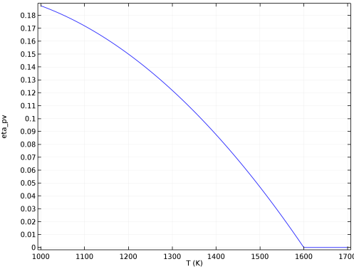
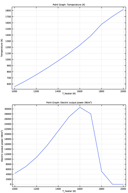
In the Settings window for Point Graph, click Replace Expression in the upper-right corner of the y-Axis Data section. From the menu, choose Component 1 (comp1)>Definitions>Variables>q_out - Electric output power - W/m².
4
In the Electric Output Power toolbar, click  Plot.
As this last plot shows, the electric output power has a maximum near 1600 K. To see the temperature distribution at this operating temperature, go back to the first plot group and change the parameter value.
Temperature (ht)
1
In the Model Builder window, under Results click Temperature (ht).
2
In the Settings window for 2D Plot Group, locate the Data section.
3
From the Parameter value (T_heater (K)) list, choose 1600.
4
In the Temperature (ht) toolbar, click  Plot.
Finally, reproduce the surface irradiation plot in Figure 8 as follows:
Mutual Surface Irradiation
1
In the Home toolbar, click  Add Plot Group and choose 1D Plot Group.
2
In the Settings window for 1D Plot Group, type Mutual Surface Irradiation in the Label text field.
3
Locate the Data section. From the Parameter selection (T_heater) list, choose From list.
4
In the Parameter values (T_heater (K)) list, select 1600.
Line Graph 1
1
Right-click Mutual Surface Irradiation and choose Line Graph.
2
3
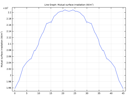
In the Settings window for Line Graph, click Replace Expression in the upper-right corner of the y-Axis Data section. From the menu, choose Component 1 (comp1)>Surface-to-Surface Radiation>Irradiation>rad.Gm_gp - Mutual surface irradiation - W/m².
4
Locate the x-Axis Data section. From the Parameter list, choose Expression.
5
In the Expression text field, type atan2(y,x)*180/pi.
Line Graph 2
1
Right-click Line Graph 1 and choose Duplicate.
2
In the Settings window for Line Graph, locate the x-Axis Data section.
3
In the Expression text field, type 360/8-atan2(y,x)*180/pi.
4
Click to expand the Title section. From the Title type list, choose None.
5
Click to expand the Coloring and Style section. From the Color list, choose Cycle (reset).
6
In the Mutual Surface Irradiation toolbar, click  Plot.
This plot of the irradiative flux in one sector of symmetry shows the shadowing effect of the mirror (at each end of the x-axis).