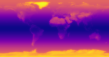
PDF

Orbit Thermal Loads
Introduction
This model demonstrates how to define Earth properties that are spatially varying on the planet. A satellite in orbit experiences solar, albedo, and planetary infrared (IR) loads, where albedo and planetary IR can vary with latitude and longitude. In this example, these inputs are read from spreadsheet and image data. The total irradiation and flux onto the satellite are evaluated over several orbits and the albedo flux is plotted over the surface of Earth.
Model Definition
To evaluate the total environmental heat loads on a satellite, it is sufficient to use a geometry that describes the outside envelope of the satellite structure. In this example, a 1U CubeSat is modeled as a 10 cm cube. A mapped mesh, with one element on each side, is sufficient to compute the incident loads since there is no shadowing.
When computing orbital heat loads, it is typical to use a two-band solar and ambient radiation model. Environmental radiation in the short-wavelength, solar band, is almost solely from the direct solar and albedo. Radiation in the long-wavelength, ambient band, is from Earth, direct solar, and albedo. The division between these bands is user-selectable and is based upon the emissive properties of the exposed materials. It is typically in the range 2–5 μm. In this example, the division is set to 2.5 μm.
The planet properties of albedo and planet flux are both functions of latitude and longitude, and since the two-band solar and ambient radiation model is used, a total of four different functions are needed.
Figure 1: Image data of the albedo in the solar band.
Results and Discussion
Figure 2 displays the albedo flux from Earth by plotting the function on the planet surface dataset, and using the solar vector. This shows how the albedo flux can vary depending upon both latitude and longitude.
Figure 2: Diffusely reflected solar band flux, the albedo.
Figure 3 shows total and per band irradiation over time.
Figure 3: Variation of the total irradiation over several orbit periods.
Figure 4 compares the total irradiation between orbits. The irradiation varies between the orbits because the planet properties depend on latitude and longitude.
Figure 4: Comparison of the total irradiation over several orbit periods.
Application Library path: Heat_Transfer_Module/Orbital_Thermal_Loads/orbit_thermal_loads
Model Instructions
From the File menu, choose New.
New
In the New window, click  Model Wizard.
Model Wizard
1
In the Model Wizard window, click  3D.
2
In the Select Physics tree, select Heat Transfer>Radiation>Orbital Thermal Loads (otl).
3
Click Add.
4
Click  Study.
5
In the Select Study tree, select Preset Studies for Selected Physics Interfaces>Orbit Thermal Loads.
6
Geometry 1
Block 1 (blk1)
1
In the Model Builder window, expand the Component 1 (comp1)>Geometry 1 node.
2
Right-click Geometry 1 and choose Block.
3
In the Settings window for Block, locate the Size and Shape section.
4
In the Width text field, type 10[cm].
5
In the Depth text field, type 10[cm].
6
In the Height text field, type 10[cm].
7
Locate the Position section. From the Base list, choose Center.
Definitions
Now, define the two functions for the albedo in the solar and ambient bands.
The albedo in the solar band is defined as a function of latitude and longitude and based upon image data.
Image Data of Solar Band Albedo
1
In the Home toolbar, click  Functions and choose Local>Image.
2
In the Settings window for Image, type Image Data of Solar Band Albedo in the Label text field.
3
Locate the File section. Click  Browse.
4
5
Click  Import.
6
In the Function name text field, type imageData.
7
Locate the Coordinates section. In the x minimum text field, type -pi.
8
In the x maximum text field, type pi.
9
In the y minimum text field, type -pi/2.
10
In the y maximum text field, type pi/2.
11
Locate the Units section. In the Arguments text field, type rad.
12
In the Function text field, type 1.
Image-Based Albedo, Solar Band
1
In the Home toolbar, click  Functions and choose Local>Analytic.
2
In the Settings window for Analytic, type Image-Based Albedo, Solar Band in the Label text field.
3
In the Function name text field, type ImageBasedAlbedoSolarBand.
4
Locate the Definition section. In the Expression text field, type imageData(Longitude,Latitude).
5
In the Arguments text field, type Latitude, Longitude.
6
Locate the Units section. In the table, enter the following settings:
7
Locate the Plot Parameters section. In the table, enter the following settings:
Constant Albedo, IR Band
1
In the Home toolbar, click  Functions and choose Local>Analytic.
In the ambient band, the albedo is set to 0.3 everywhere on the planet.
2
In the Settings window for Analytic, type Constant Albedo, IR Band in the Label text field.
3
In the Function name text field, type ConstantAlbedo_IR_Band.
4
Locate the Definition section. In the Expression text field, type 0.3.
5
In the Arguments text field, type Latitude, Longitude.
Now, define the planet IR flux in the ambient band. It is defined from tabular data and varies with latitude only. The planet IR flux function in the solar band is zero.
IR Flux w.r.t. Latitude
1
In the Home toolbar, click  Functions and choose Local>Interpolation.
2
In the Settings window for Interpolation, locate the Definition section.
3
4
In the Label text field, type IR Flux w.r.t. Latitude.
5
Locate the Units section. In the Function table, enter the following settings:
6
In the Argument table, enter the following settings:
Planetary Flux, IR Band
1
In the Home toolbar, click  Functions and choose Local>Analytic.
2
In the Settings window for Analytic, type Planetary Flux, IR Band in the Label text field.
3
In the Function name text field, type PlanetaryFlux_IR_Band.
4
Locate the Definition section. In the Expression text field, type int1(Latitude*90/pi).
5
In the Arguments text field, type Latitude, Longitude.
6
Locate the Units section. In the table, enter the following settings:
Integration 1 (intop1)
1
In the Definitions toolbar, click  Nonlocal Couplings and choose Integration.
An integration operator is added to integrate the external irradiation over the spacecraft boundaries.
2
In the Settings window for Integration, type intopAll in the Operator name text field.
3
Locate the Source Selection section. From the Geometric entity level list, choose Boundary.
4
From the Selection list, choose All boundaries.
Orbital Thermal Loads (otl)
Sun Properties 1
The Sun vector and solar flux are set to correspond to the summer solstice.
1
In the Model Builder window, under Component 1 (comp1)>Orbital Thermal Loads (otl) click Sun Properties 1.
2
In the Settings window for Sun Properties, locate the Sun Properties section.
3
From the Sun direction list, choose Summer solstice.
Planet Properties 1
1
In the Model Builder window, click Planet Properties 1.
2
In the Settings window for Planet Properties, locate the Planet Properties section.
3
Find the Planet initial position subsection. From the Planet longitude at start time list, choose Longitude at subspacecraft point.
Select the previously defined functions for the albedo and planet IR flux depending on latitude and longitude.
4
Locate the Radiative Properties section. From the Geographic position dependence list, choose Latitude and longitude.
5
From the fα0(lat,long) list, choose User defined for each band.
6
7
From the fq0,IR(lat,long) list, choose User defined for each band.
8
Orbital Parameters 1
A circular orbit is defined at 400 km altitude, inclination of 50°, and local time at ascending node set to 15h.
1
In the Model Builder window, click Orbital Parameters 1.
2
In the Settings window for Orbital Parameters, locate the Orbital Parameters section.
3
From the Orbit type list, choose Circular.
4
In the R text field, type otl.R_planet+400[km].
5
In the i text field, type 50[deg].
6
From the Ascending node list, choose Local time at ascending node.
7
In the tΩ text field, type 15[h].
Spacecraft Orientation 1
The orientation of the satellite is such that the primary direction points towards Earth. The satellite is slowly rotating about its primary axis, so the secondary axis can be any vector that is not parallel to nadir. In this case the default setting, of the +X direction corresponding to the direction of travel, is used.
1
In the Model Builder window, click Spacecraft Orientation 1.
2
In the Settings window for Spacecraft Orientation, locate the Spacecraft Orientation section.
3
Find the Rotations subsection. From the Rotation about primary axis list, choose Angular rate.
4
In the ω text field, type 2*360[deg]/otl.T_orbit.
Generate Events Interface 1
In order to handle the passing of the spacecraft through the eclipse, an Events interface is necessary and should always be added when using the Orbital Thermal Loads physics.
1
In the Model Builder window, click Generate Events Interface 1.
2
In the Settings window for Generate Events Interface, locate the Generate Events Interface section.
3
Click Create New.
Diffuse Surface 1
Now, define the radiative properties of the different boundaries.
1
In the Model Builder window, click Diffuse Surface 1.
2
In the Settings window for Diffuse Surface, locate the Surface Emissivity section.
3
From the ε list, choose User defined for each band.
4
Diffuse Surface 2
1
In the Physics toolbar, click  Boundaries and choose Diffuse Surface.
2
In the Settings window for Diffuse Surface, locate the Boundary Selection section.
3
Click  Paste Selection.
4
In the Paste Selection dialog box, type 1 2 5 6 in the Selection text field.
5
6
In the Settings window for Diffuse Surface, locate the Surface Emissivity section.
7
From the ε list, choose User defined. In the associated text field, type 0.95.
Mesh 1
A mapped mesh, with one element on each side, is sufficient to compute the incident loads since there is no shadowing.
Swept 1
In the Mesh toolbar, click  Swept.
Size
1
In the Model Builder window, click Size.
2
In the Settings window for Size, locate the Element Size section.
3
Click the Custom button.
4
Locate the Element Size Parameters section. In the Maximum element size text field, type 0.1.
5
Click  Build All.
Study 1
Step 1: Orbit Thermal Loads
1
In the Model Builder window, under Study 1 click Step 1: Orbit Thermal Loads.
2
In the Settings window for Orbit Thermal Loads, locate the Study Settings section.
3
In the Output orbit times text field, type range(0,0.01,5).
4
Click to expand the Values of Dependent Variables section. In the Home toolbar, click  Compute.
Results
Orbit Visualization (otl)
Modify the default Orbit Visualization plot to display the albedo flux on the planet.
1
In the Model Builder window, expand the Orbit Visualization (otl) node.
Eclipse
1
In the Model Builder window, expand the Results>Orbit Visualization (otl)>Eclipse node, then click Eclipse.
2
In the Settings window for Surface, locate the Coloring and Style section.
3
From the Color list, choose Custom.
4
5
Click Define custom colors.
6
7
Click Add to custom colors.
8
Click Show color palette only or OK on the cross-platform desktop.
Transparency 1
1
In the Model Builder window, click Transparency 1.
2
In the Settings window for Transparency, locate the Transparency section.
3
In the Transparency text field, type 0.2.
Albedo Flux
1
In the Model Builder window, right-click Orbit Visualization (otl) and choose Surface.
2
In the Settings window for Surface, type Albedo Flux in the Label text field.
3
Locate the Expression section. In the Expression text field, type -ImageBasedAlbedoSolarBand(Latitude, Longitude)*otl.sup1.q0s*(x*otl.SVX_ECS+y*otl.SVY_ECS+z*otl.SVZ_ECS).
4
Locate the Coloring and Style section. Click  Change Color Table.
5
In the Color Table dialog box, select Rainbow>RainbowDark in the tree.
6
Filter 1
1
Right-click Albedo Flux and choose Filter.
2
In the Settings window for Filter, locate the Element Selection section.
3
In the Logical expression for inclusion text field, type x*otl.SVX_ECS+y*otl.SVY_ECS+z*otl.SVZ_ECS<0.
Transparency 1
1
In the Model Builder window, right-click Albedo Flux and choose Transparency.
2
In the Settings window for Transparency, locate the Transparency section.
3
In the Transparency text field, type 0.2.
Albedo Flux
1
In the Model Builder window, click Albedo Flux.
2
In the Orbit Visualization (otl) toolbar, click  Plot.
Plot the evolution of total and per band irradiation over time.
Total and Per Band Irradiation Over Time
1
In the Home toolbar, click  Add Plot Group and choose 1D Plot Group.
2
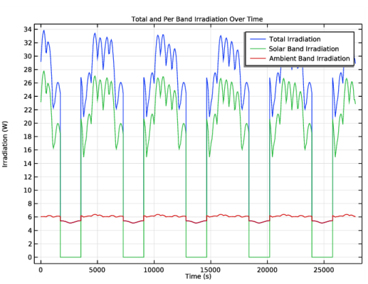
In the Settings window for 1D Plot Group, type Total and Per Band Irradiation Over Time in the Label text field.
3
Locate the Plot Settings section.
4
Select the y-axis label check box. In the associated text field, type Irradiation (W).
5
Click to expand the Title section. From the Title type list, choose Label.
Global 1
1
Right-click Total and Per Band Irradiation Over Time and choose Global.
2
In the Settings window for Global, locate the y-Axis Data section.
3
4
In the Total and Per Band Irradiation Over Time toolbar, click  Plot.
Plot the evolution of total irradiation on each orbit period.
Total Irradiation, Periodic Comparison
1
In the Home toolbar, click  Add Plot Group and choose 1D Plot Group.
2
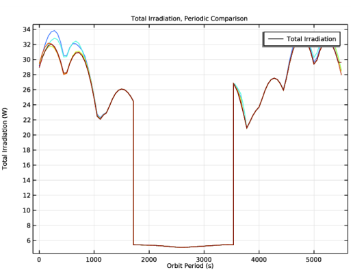
In the Settings window for 1D Plot Group, type Total Irradiation, Periodic Comparison in the Label text field.
3
Locate the Plot Settings section.
4
Select the x-axis label check box. In the associated text field, type Orbit Period (s).
5
Locate the Title section. From the Title type list, choose Label.
Global 1
1
Right-click Total Irradiation, Periodic Comparison and choose Global.
2
In the Settings window for Global, locate the y-Axis Data section.
3
4
Locate the x-Axis Data section. From the Parameter list, choose Expression.
5
In the Expression text field, type mod(t,otl.T_orbit).
Filter 1
1
Right-click Global 1 and choose Filter.
2
In the Settings window for Filter, locate the Line Segment Selection section.
3
Clear the Decreasing x check box.
Color Expression 1
1
In the Model Builder window, right-click Global 1 and choose Color Expression.
2
In the Settings window for Color Expression, locate the Expression section.
3
In the Expression text field, type ceil(t/otl.T_orbit).
4
Select the Description check box. In the associated text field, type Orbit Number.
5
Locate the Coloring and Style section. Clear the Color legend check box.
6
In the Total Irradiation, Periodic Comparison toolbar, click  Plot.
Total Irradiation, Periodic Comparison
1
In the Model Builder window, under Results click Total Irradiation, Periodic Comparison.
2
In the Settings window for 1D Plot Group, locate the Legend section.
3
Clear the Show legends check box.
Finally, add an evaluation group to get the time-averaged total environmental irradiation.
Average of Total Irradiation Over Time
1
In the Results toolbar, click  Evaluation Group.
2
In the Settings window for Evaluation Group, type Average of Total Irradiation Over Time in the Label text field.
3
Locate the Data section. From the Time selection list, choose First.
4
Locate the Transformation section. Select the Transpose check box.
5
Click to expand the Format section. From the Include parameters list, choose Off.
Global Evaluation 1
1
Right-click Average of Total Irradiation Over Time and choose Global Evaluation.
2
In the Settings window for Global Evaluation, locate the Expressions section.
3
4
In the Average of Total Irradiation Over Time toolbar, click  Evaluate.